Chapter 1.1 — The Memory Hierarchy That Matters¶
In one line: An A100 can do 153 floating-point operations in the time it takes to fetch one byte, and LLM decode gives it about one — so every serving decision in this book is really a decision about bytes.
| Part | I — The Machine |
| Chapter | 1.1 |
| Time | ~110 min |
| Prereqs | 1.0 GPU execution model |
| Notation | \(P_{peak}\), \(B_{mem}\), \(I_{ridge}\), \(M_w\), \(N\), \(s\) |
| Status | built |
Where we are
Chapter 1.0 gave you SMs, warps, occupancy and coalescing — how work is scheduled. This chapter answers whether that work ever gets any data: how bytes reach the arithmetic units, and how fast. It ends with a hard floor on decode speed that no kernel can break. Chapter 1.2 turns the single ratio derived here into a diagnostic you can point at any kernel, and nothing in Part II — least of all the KV cache — makes economic sense until this arithmetic is reflexive.
Why this matters¶
Load Llama-3.1-8B onto an A100 80 GB and you have used 14.96 GiB of an 80 GiB card. The natural conclusion — plenty of room — is correct and completely useless. Capacity was never going to be your problem at 8 B parameters. Bandwidth is. An A100 80 GB SXM is rated at 312 TFLOP/s of dense bf16 tensor-core throughput and 2.039 TB/s of HBM bandwidth. Divide one by the other:
To keep the tensor cores saturated, a kernel must perform 153 floating-point operations for every byte it pulls from HBM. A batch-one decode step performs roughly one: each bf16 weight is two bytes and contributes one multiply and one add, then is never touched again for the rest of that step.
You are running the machine at about 0.65% of its advertised compute, and no kernel rewrite fixes a deficit of 153×. This is not an implementation failure but the structure of autoregressive decoding meeting the structure of modern silicon, and LLM serving is the discipline of pushing that ratio up.
The sentence to remember
Capacity tells you whether the model fits. Bandwidth tells you how fast it runs. Almost every performance surprise in this book comes from someone who checked the first and assumed the second.
The mental model¶
Picture a workshop. Every worker has a small bench in arm's reach, and one shared warehouse holds essentially all the material. Throughput is decided by how often a worker walks to the warehouse.
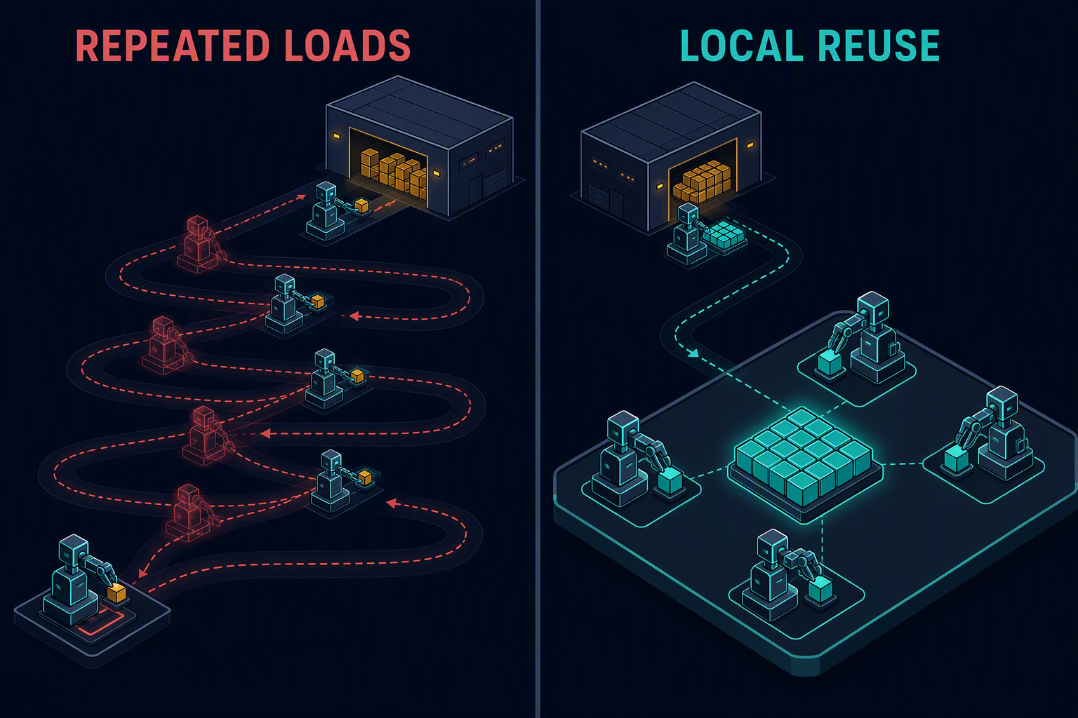
Figure 1.1.1 — Every trip to the warehouse is a trip not spent working. Reuse is the only thing that makes the trip worth taking.
A GPU does not have one bench; it has a graded sequence of them, and the trade is brutal at every step.
flowchart TB
    R["Registers — per thread<br/>≈27 MiB device-wide"]
    S["Shared memory / L1 — per SM<br/>192 KiB × 108 SMs ≈ 20 MiB"]
    L["L2 cache — device-wide<br/>40 MB"]
    H[("HBM — device capacity<br/>80 GiB @ 2.039 TB/s")]
    C[("Host DRAM — over PCIe<br/>≈64 GB/s")]
    R --> S --> L --> H --> C
    R -.->|"spills"| H
Figure 1.1.2 — Moving down buys capacity and costs locality. The dotted edge catches people out: register pressure does not degrade gracefully into L1, it falls all the way to HBM.
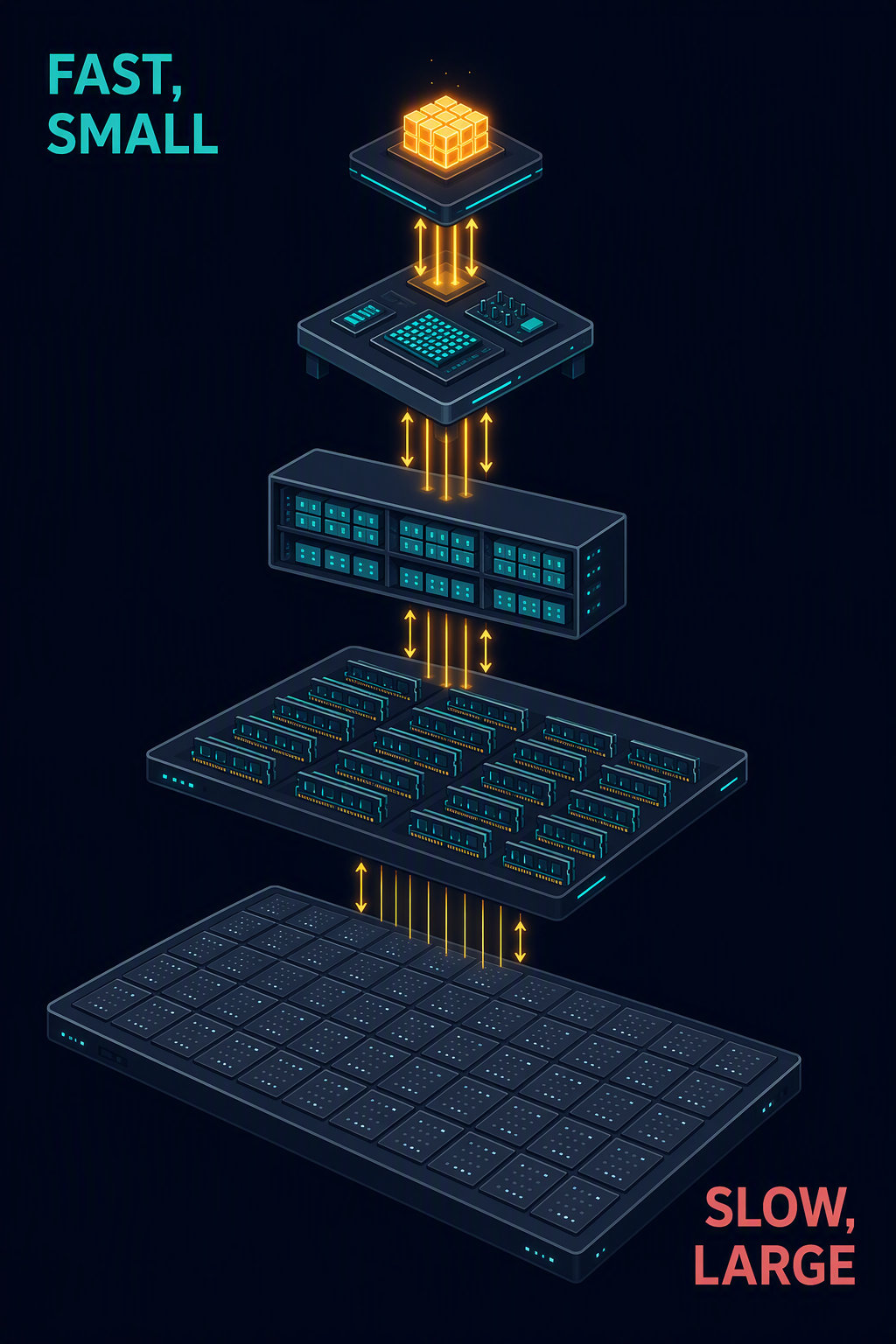
Figure 1.1.3 — The fastest storage is tiny and private; every larger tier is easier to fill and more expensive to reach.
Put the running example against those tiers. Llama-3.1-8B's weights are 14.96 GiB. The entire GPU has about 20 MiB of shared memory, 27 MiB of register file and 40 MB of L2 — 85 MiB of on-chip storage, roughly one thousandth of HBM's capacity. The weights alone are 400× larger than L2 and 750× larger than every SM's shared memory combined; one SM's 192 KiB holds 98,304 bf16 values, or one weight in 82,000.
There is no version of "keep the model on chip". So stop asking where a tensor lives — it is allocated in HBM while its active tile sits in L2, L1, shared memory and registers at different instants. Ask instead: how many bytes cross the HBM boundary per useful operation? That is the only number performance responds to.
The mechanism¶
Four properties, routinely confused¶
| Property | Answers | The mistake it invites |
|---|---|---|
| Capacity | How many bytes fit at this tier? | Assuming an 80 GiB card can serve an 80 GiB model |
| Bandwidth | How many bytes cross this boundary per second? | Quoting the spec sheet as achieved bandwidth |
| Latency | How long does one dependent access wait? | Believing enough threads make latency vanish |
| Scope | Which threads can see this data? | Staging into shared memory when one thread reuses it |
Capacity and bandwidth decide serving economics, and they fail differently. Capacity failure is loud:
an allocation raises OOM. Bandwidth failure is silent — everything works, nvidia-smi shows 100%
utilisation, and throughput is a third of what the FLOP count promised. A bigger card fixes the first;
only a faster card, or less traffic, fixes the second.
Registers: fast, finite, quietly dangerous¶
Registers are the only storage the arithmetic units read directly — 256 KiB per SM, 65,536 32-bit registers, 255 maximum per thread. The trap is that the file is shared across all resident threads. Ask for more registers per thread and fewer warps fit, so there is less independent work to hide memory latency with (Chapter 1.0's occupancy). Push further and the compiler spills to "local memory", which despite the name is device memory. You reached for the fastest tier and landed on the slowest.
The classic reversal
A kernel gets slower after you cache more values in registers. Two mechanisms, and you must distinguish them: occupancy loss (fewer resident warps, so latency stops being hidden) or spilling (the values you "cached" now round-trip through HBM). Check the compiler's per-thread register count and the profiler's spill-store/spill-load counters. Guessing here wastes days.
Shared memory, L1 and L2: where reuse is manufactured¶
Shared memory is programmer-managed scratch visible to every thread in a block, sharing a 192 KiB unified block with L1 per SM. It is the tier that makes matrix multiplication viable: a tiled matmul loads a tile of \(A\) and a tile of \(B\) once, synchronises, and performs many fused multiply-adds against those resident values before moving on. The FLOP count is unchanged; HBM traffic drops by roughly the tile dimension.
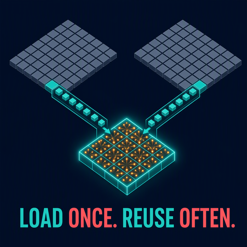
Figure 1.1.4 — One HBM load only pays for itself when the on-chip tile serves many operations. The tile size is the arithmetic intensity.
The device-wide 40 MB L2 catches reuse across thread blocks and consecutive kernels and absorbs hot metadata like block tables. It is also the commonest source of fraudulent benchmark numbers, because a working set under 40 MB never touches HBM and will happily report bandwidth above spec. It is not a storage strategy: in real serving, weights, KV pages, activations and co-tenant kernels contend for the same 40 MB.
HBM: the tier that sets the ceiling¶
HBM2e on the A100 delivers 2.039 TB/s across 80 GiB — roughly twenty times a well-configured server's DRAM. Relative to the compute beside it, it is starving, which is what Equation 1.1 said.
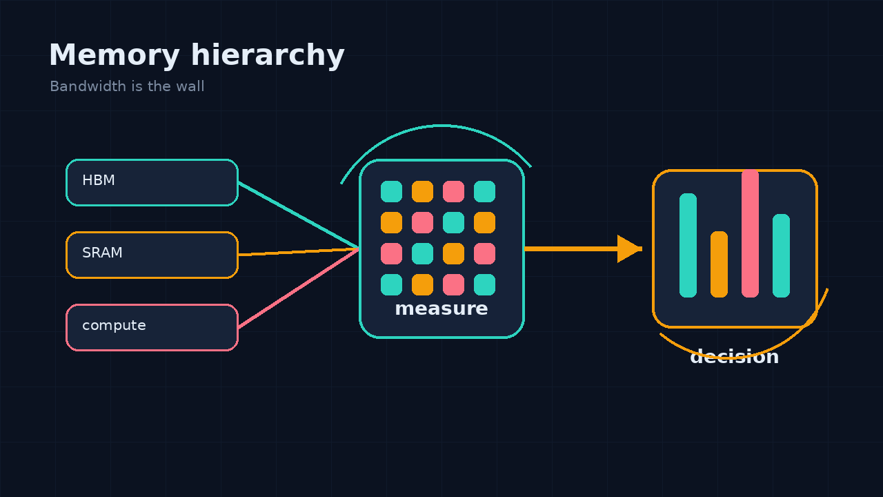
Figure 1.1.5 — Compute has grown far faster than the pipe that feeds it. The narrow throat between the columns is where every decode step spends its life.
Worked example — the floor on Llama-3.1-8B decode
At batch 1 a decode step must read every weight the model has: every layer participates in producing one token, and each weight multiplies exactly one activation vector. There is no reuse.
One token per 7.9 ms is ≈ 127 tokens per second, and that is the ceiling — not a benchmark, a bound. It assumes perfect bandwidth utilisation, zero KV cache traffic, zero activation traffic, zero launch overhead and infinitely fast tensor cores. Every assumption is generous. So if someone shows you 300 tok/s at batch 1 on one A100 for a bf16 8 B model, one of three things is true: the batch is not 1, the weights are not bf16, or the measurement is wrong. There is no fourth option.
Equation 1.2 is the emotional centre of this book. Decode speed is set by a division you can do in your head, and there are only three ways to move it: shrink the numerator (quantisation, Skill 03), grow the denominator (a faster card), or amortise the numerator across more tokens (batching, Skill 01). The third is free, which is why every serving engine you meet is fundamentally a batching machine wearing an HTTP interface.
The same arithmetic explains prefill's opposite personality. A 2,000-token prompt reads the same 16.06 GB of weights once and does 2,000 tokens' work with it. Intensity jumps from ≈1 to ≈2,000 FLOP/byte, past the ridge point of 153, and prefill becomes compute-bound. Same weights, same card, opposite bottleneck — the split Chapter 2.4 builds a scheduling discipline on.
Why FlashAttention had to be invented¶
Weights are not the only thing crossing the boundary. Standard attention computes \(S = QK^\top\), softmaxes it to \(P\), then computes \(PV\). For one head over \(T\) tokens, \(S\) is \(T \times T\) — not a weight, not an output, pure scratch. A naive implementation materialises it in HBM, reads it back for softmax, writes \(P\), and reads \(P\) again.
Worked example — the cost of materialising the score matrix
One attention head of Llama-3.1-8B at \(T = 8192\), scores accumulated in fp32.
- Inputs: \(Q\), \(K\), \(V\) are each \(8192 \times 128\) in bf16 = 2.1 MiB, 6.3 MiB total.
- Intermediate: \(S\) is \(8192 \times 8192\) in fp32 = 268 MB.
The scratch is over forty times larger than the data that produced it. Round-tripping it (write \(S\), read \(S\), write \(P\), read \(P\)) costs roughly 1 GB of HBM traffic per head, per layer, per forward pass — against 16 GB for the model's whole weight set. Multiply by 32 heads and 32 layers and attention, not the weights, owns the memory system. The cost is also quadratic in \(T\): double the context and this term quadruples while the weight term does not move.
FlashAttention's insight is that \(S\) never needs to exist all at once. Softmax can be computed incrementally: process \(K\) and \(V\) in blocks, keep a running maximum and running sum, and rescale the partial output as each block arrives. The matrix is produced one tile at a time, consumed in shared memory, discarded. The tiling fits the hardware exactly: with \(B_r = B_c = 64\) and \(d_h = 128\) in bf16, the \(Q\), \(K\) and \(V\) tiles are 16 KiB each and the \(64 \times 64\) fp32 score tile another 16 KiB — 64 KiB against the SM's 192 KiB budget, with room for double buffering. The algorithm was designed backwards from the size of the scratchpad.
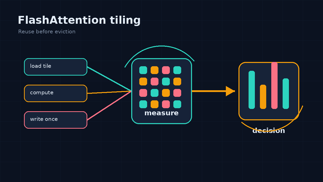
Figure 1.1.6 — The score matrix is real, computed and used; it simply never lands in HBM. Traffic collapses to \(Q\), \(K\), \(V\) and the output, plus a modest re-read factor.
FlashAttention changes no mathematics — outputs match the naive kernel up to floating-point associativity. It is purely a memory-hierarchy optimisation, worth 2–4× on long context.
The KV cache is a bandwidth problem¶
Chapter 2.2 shows Llama-3.1-8B costs 128 KiB of KV cache per token, and it is tempting to file that as capacity. It is also traffic, and traffic usually bites first: every decode step reads the entire live cache, because attention at position \(t\) compares against all \(t\) stored keys and mixes all \(t\) stored values. Weights are read once and shared across the batch; cache is read once per sequence and shared with nobody.
Sixty users at 8 K context hold 60 GiB of cache — four times the weight traffic, on the same 2.039 TB/s pipe, every step. Batching amortises the first term and does nothing to the second. That is why GQA, KV quantisation and shorter contexts are bandwidth optimisations that happen to save capacity too.
flowchart LR
    W["Weights<br/>16.06 GB<br/>read once per step"] --> BUS
    KV["KV cache<br/>0.5 GiB per 4K sequence<br/>read once per sequence"] --> BUS
    A["Activations<br/>small at decode"] --> BUS
    BUS{{"HBM boundary<br/>2.039 TB/s"}} --> SM["On-chip: L2 → L1/shared → registers"]
    SM --> TC["Tensor cores<br/>312 TFLOP/s"]
Figure 1.1.7 — Everything a decode step needs squeezes through one 2.039 TB/s boundary. Batching improves the weight arrow's payoff and does nothing to the cache arrow, which multiplies with every user.
In practice¶
Never trust the spec sheet as an achievable number. A good copy kernel on a healthy A100 sustains 80–90% of published HBM bandwidth. The gap is structural: ECC overhead, DRAM refresh, row activation, imperfect access patterns, and vendor figures being pin-rate ceilings.
Worked example — what the 80–90% gap costs you
Redo Equation 1.2 at a realistic 85% of peak, \(0.85 \times 2.039 = 1.733\) TB/s:
A 17% haircut on your entire latency budget, found before you write a line of serving code. Two A100s in the same rack can differ by more than 10% under different power caps, thermal conditions or ECC settings, and an SXM part is not a PCIe part. Benchmark your own card; do not quote a datasheet.
Audit units before you audit performance. Vendors publish bandwidth in decimal GB/s (\(10^9\)); allocators report capacity in binary GiB (\(2^{30}\)). Mixing them injects a 7.4% error before you measure anything — the same magnitude as the effects you are hunting.
Count traffic at the boundary that limits you. If a fused kernel keeps an intermediate in registers, do not charge it to HBM; if two kernels materialise and reload it, do. That is why fusion helps a memory-bound operation with no change in FLOP count. Report median with p10/p90, never the best sample, because one fast iteration usually means you measured cache.
On newer silicon
Hopper (H100, SM 9.0) moves to HBM3 at ~3.35 TB/s and H200 to HBM3e at ~4.8 TB/s, and adds distributed shared memory, letting thread blocks in a cluster read each other's shared memory directly — a new tier between L1 and L2 that changes which tiling strategies are possible. The Tensor Memory Accelerator handles bulk asynchronous transfers Ampere must do with threads. We cannot run any of this. The baseline here is A100 SXM (SM 8.0) and every success criterion in this book is reachable there. Note that Equation 1.1's ratio worsens on H100 — compute grew faster than bandwidth again — but keep these features out of an Ampere capacity plan.
Failure modes¶
| Symptom | Cause | Fix |
|---|---|---|
| Measured bandwidth exceeds the published HBM spec | The working set fit in the 40 MB L2, or read+write bytes were counted inconsistently | Raise --size-mib until the curve plateaus; state the traffic convention (a copy moves each byte twice) |
| Timings implausibly close to zero | The host timer stopped before the asynchronous CUDA work finished | torch.cuda.synchronize() immediately before reading the clock, or use CUDA events |
| Bandwidth degrades across iterations | Thermal or power throttling, or a competing process on the device | Capture clocks, power and temperature with 1.5; rerun on a quiet card |
| Tuned kernel gets slower after enlarging the tile | Register pressure cut occupancy, or the compiler started spilling to local (device) memory | Check per-thread register count and profiler spill counters; shrink the tile or the thread-local state |
| Model fits by parameter bytes but still OOMs | CUDA context, workspaces, activations, KV cache and fragmentation also consume HBM | Build a full budget with explicit headroom; parameters are a lower bound, never the total |
| Throughput far below the FLOP estimate while the GPU shows 100% "utilisation" | That counter means a kernel is resident, not the arithmetic units are busy — you are bandwidth-bound | Compute arithmetic intensity against Equation 1.1; use 1.2 |
| Decode latency scales with context length despite a KV cache | Cache reads are HBM traffic and grow linearly with \(T\) (Equation 1.3) | Attack cache bytes — GQA, KV quantisation, shorter contexts — not weight quantisation |
Do it¶
Run the bandwidth artifact with a buffer comfortably larger than the 40 MB L2, passing the published peak for your exact SKU:
The accounting line worth reading is # [1]: a copy moves each byte twice, one read and one write, so
the numerator is 2 * source.nbytes. Report the source size alone and you understate traffic by half.
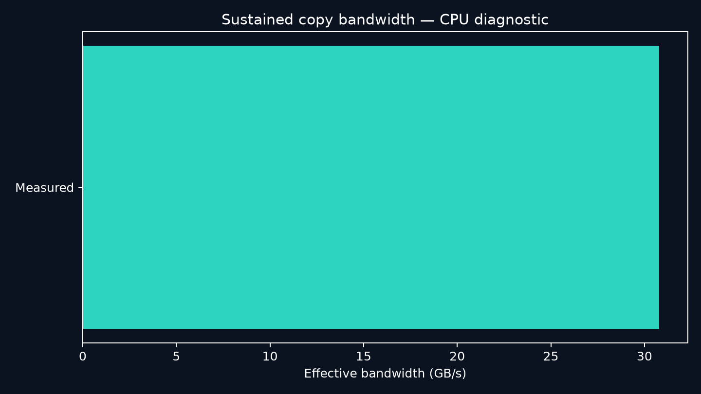
Figure 1.1.8 — The committed chart is the CPU diagnostic run, not HBM evidence: latest.json
records "measurement_scope": "host-memory diagnostic" and a median of 30.8 GB/s. A valid GPU result
reports "measurement_scope": "HBM" and names the CUDA device. Never quote the diagnostic as bandwidth.
Success criterion. Three things, all objective:
- Sweep 4, 64, 256 and 1024 MiB. Small sizes are inflated by cache and launch overhead; the curve must reach a visible plateau, and the plateau — not the best sample — is your number.
- Three repeated large-buffer medians agree within 5%.
- Your measured percentage of peak lands in the 80–90% band and you can explain the gap from traffic accounting and observed clocks. If it lands at 40%, finding out why is the exercise.
Carry the plateau into LAB-M1, where the misleading small-buffer run is laid as a trap you have to diagnose.
Summary¶
- On-chip storage totals ≈85 MiB against 80 GiB of HBM; the weights are 400× larger than L2. Nothing stays on chip, so the only question is work extracted per byte.
- \(I_{ridge} \approx 153\) FLOP/byte on an A100; batch-1 decode delivers about 1. Closing that gap is the entire serving discipline.
- Weight traffic alone floors decode at 7.9 ms per step, ≈127 tok/s for bf16 Llama-3.1-8B at batch 1. No kernel beats it; batching is the only free way around it.
- FlashAttention is a pure memory-hierarchy optimisation: hold the score matrix in a 64 KiB tile inside the SM's 192 KiB instead of round-tripping 268 MB through HBM.
- Spec bandwidth is a ceiling, not an expectation. Plan for 80–90% and measure your own card.
Key terms¶
HBM · bandwidth-bound · arithmetic intensity · occupancy · coalesced access · KV cache
Exercises¶
Recall
- Name the four on-device tiers in order and state which threads can see each one.
- State Equation 1.1 in words, give its A100 value, and say what a kernel below it is called.
- Why is
nvidia-smiat 100% utilisation not evidence that the tensor cores are busy?
Derive
- A copy kernel reads 800 MiB and writes 800 MiB in 1.2 ms. What belongs in the effective-bandwidth numerator, and what is the result in GB/s?
- Compute the batch-1 decode floor for a 70 B model in bf16 on the same A100, then say what the number means and why the model does not actually fit.
- At what batch size does weight traffic stop dominating for Llama-3.1-8B, if every sequence holds 4 K tokens of KV cache? Use Equation 1.3.
Design
- Your service runs Llama-3.1-8B on one A100 80 GB. Batch-1 decode measures 96 tok/s. Product wants 200 tok/s per user. Decide whether that is achievable; if not, say exactly what must change and what each option costs.
Worked solutions
**1.** Registers (one thread) → shared memory / L1 (all threads in a block, 192 KiB per SM) → L2 (device-wide, 40 MB) → HBM (device-wide, 80 GiB, and the boundary every performance argument is really about). Host DRAM sits beyond it across PCIe. **2.** $I_{ridge} = P_{peak} / B_{mem}$: the FLOPs a kernel must do per byte of HBM traffic to keep the arithmetic units saturated. On an A100 80 GB, $312 / 2.039 \approx 153$ FLOP/byte. A kernel below it is **bandwidth-bound** — it finishes when the bytes arrive, not when the maths completes. **3.** That counter reports the fraction of sampled intervals in which *at least one kernel was resident*. A kernel stalled on every memory access for its entire life scores 100%. It is a device-occupancy signal, not an arithmetic-throughput one. **4.** Both directions count: 800 MiB read *and* 800 MiB written, so the numerator is 1,600 MiB $= 1.678 \times 10^9$ bytes. Over $1.2 \times 10^{-3}$ s that is **≈ 1,398 GB/s**. Charging only the source size reports 699 GB/s and makes a healthy card look broken. **5.** $M_w = 140\ \text{GB}$, so $t_{floor} \approx 68.7$ ms — **≈ 14.6 tok/s**, below comfortable reading speed, from bandwidth alone. It is also academic on one card: 140 GB does not fit in 80 GiB (= 85.9 GB), so you need at least two A100s and therefore tensor parallelism, which adds all-reduce traffic. Capacity and bandwidth fail together here, and they are different failures. **6.** Weight traffic is fixed at 16.06 GB per step; cache traffic is $C \times 4096 \times 128$ KiB $= C \times 0.537$ GB. Equal at $C \approx \mathbf{30}$. Below batch 30 weights dominate and weight quantisation is your best move; above it the cache dominates and weight quantisation is rearranging deck chairs. Most production serving runs above that line. **7.** Not achievable, and the derivation is short enough to do in the meeting. Equation 1.2 caps batch-1 decode at 127 tok/s with *perfect* bandwidth, so the measured 96 tok/s is 76% of the floor — a healthy result, not a bug. 200 tok/s needs a 5 ms step, demanding 3.2 TB/s, more than an A100 physically has. Ranked by leverage per unit of pain: 1. **Quantise the weights.** W8A8 halves $M_w$ to 8.03 GB, moving the floor to 3.9 ms (≈254 tok/s) with a realistic outcome near 190. Price: accuracy validation, and int4 decode is dequantisation-heavy so you will not see a full 4×. The only option that changes the physics on hardware you own. 2. **Speculative decoding.** Several tokens per weight-read pass — it attacks *amortisation*, not size. Price: a draft model, a verification step, and gains that collapse at low acceptance rates. 3. **A faster card.** H100 at ~3.35 TB/s reaches the target. Price: money, and Equation 1.1's ratio is *worse* there, so you meet this wall again one model size up. 4. **Renegotiate.** 96 tok/s is roughly six times reading speed; the 200 is often a proxy for time-to-first-token, a prefill problem with different fixes ([Chapter 2.4](M2T4-prefill-vs-decode.md)). What you must *not* do is raise batch size and report the improvement. Batching lifts aggregate throughput while leaving per-user tokens per second flat or slightly worse, and answering a per-user latency question with an aggregate throughput number is the most common dishonesty in this field.Going deeper¶
- NVIDIA A100 Tensor Core GPU Architecture — source of the 40 MB L2 and 192 KiB unified L1/shared figures
- FlashAttention: Fast and Memory-Efficient Exact Attention with IO-Awareness — §3 is the tiling argument in full, with the HBM-access bound
- CUDA C++ Programming Guide — Memory Hierarchy — authoritative scope and lifetime rules per tier
- CUDA C++ Best Practices — Memory Optimizations — coalescing, occupancy and spill diagnosis
- Data Movement Is All You Need — systematic transformer traffic analysis; read it as method, not numbers
Next: Chapter 1.2 — Reading the Roofline turns Equation 1.1's single ratio into a two-line graph you can plot any kernel onto, and a repeatable procedure for deciding whether to attack bytes or FLOPs.