Chapter 1.4 — Multi-GPU Plumbing

In one line: A second GPU halves the weights each device must read and then hands you a bill for every layer of every token — and whether that trade wins is decided by the wires in the chassis, not by the number of GPUs in it.

Part	I — The Machine
Chapter	1.4
Time	~120 min
Prereqs	1.1 Memory hierarchy, 1.3 Precision formats
Notation	\(B\), \(d\), \(L\), \(s\), \(M_w\), \(B_{mem}\); this chapter borrows \(N\) for rank count, and writes parameter count out in full
Status	draft

Where we are

Chapter 1.3 shrank the model by changing how each number is encoded. This chapter shrinks it a different way — by cutting the weight matrices in half and putting each half on its own GPU — and asks the only question that matters about that idea: does it actually go faster? The answer depends on a communication cost model you will use again in 1.5 (toolchain diagnostics), where reading the machine's topology becomes a diagnostic reflex rather than an optimisation.

---

Why this matters

You have Llama-3.1-8B in bf16. It occupies 14.96 GiB. Your A100 has 80 GB. Nobody needs tensor parallelism here.

And yet teams reach for --tensor-parallel-size 2 anyway, because decode is bandwidth-bound: every token forces a full read of all 16.06 × 10⁹ bytes of weights out of HBM, and at a realistically achievable 1.5 TB/s that is 10.7 ms per token. Split the weights across two GPUs and each reads half — 5.35 ms. Twice the tokens per second for twice the hardware: cost-neutral, latency-halving. An attractive story.

It is also wrong by an amount that depends entirely on what is soldered between the two cards. An A100 SXM has twelve NVLink 3.0 links at 50 GB/s bidirectional each — 600 GB/s aggregate to its neighbours. A PCIe Gen4 ×16 slot gives 64 GB/s bidirectional, shared with everything else on that root complex. A ~10× gap — and the two machines are indistinguishable in nvidia-smi -L, in your Dockerfile, and in your launch command.

The sentence to remember

Tensor parallelism's primary justification is fitting a model that does not fit on one GPU. Its secondary benefit — lower latency — is workload- and topology-dependent, and on the wrong chassis it is negative. Never assume the second one; measure it.

---

The mental model

Splitting a layer across GPUs is split, compute, exchange, continue.

Cut a weight matrix into \(N\) shards, one per device. Every device multiplies the same input by its own shard, producing a partial result — numerically incomplete, useless alone. Before the next operation can run, those partials must be combined and the answer made available everywhere.

Four terms carry the chapter. A rank is one participating process, normally pinned to one GPU. The world size \(N\) is how many ranks are in the job. A shard is the slice of a tensor one rank owns. A collective is a coordinated operation in which every rank participates by the same rule; NCCL is NVIDIA's implementation of them.

flowchart LR
    X[Input activation<br/>replicated on all ranks] --> S0[Rank 0<br/>shard of W]
    X --> S1[Rank 1<br/>shard of W]
    S0 --> P0[Partial result]
    S1 --> P1[Partial result]
    P0 --> AR{{All-reduce}}
    P1 --> AR
    AR --> Y[Complete activation<br/>on all ranks]
    Y --> NX[Next layer:<br/>repeat]

Figure 1.4.1 — The collective sits on the critical path. Nothing downstream of it can start until every rank has finished its half and the exchange has completed.

That is the whole game. The exchange is not overlapped work off to the side; in the simplest tensor-parallel implementation it is a synchronisation barrier in the middle of every layer. Whatever it costs, you pay it \(2L\) times per token.

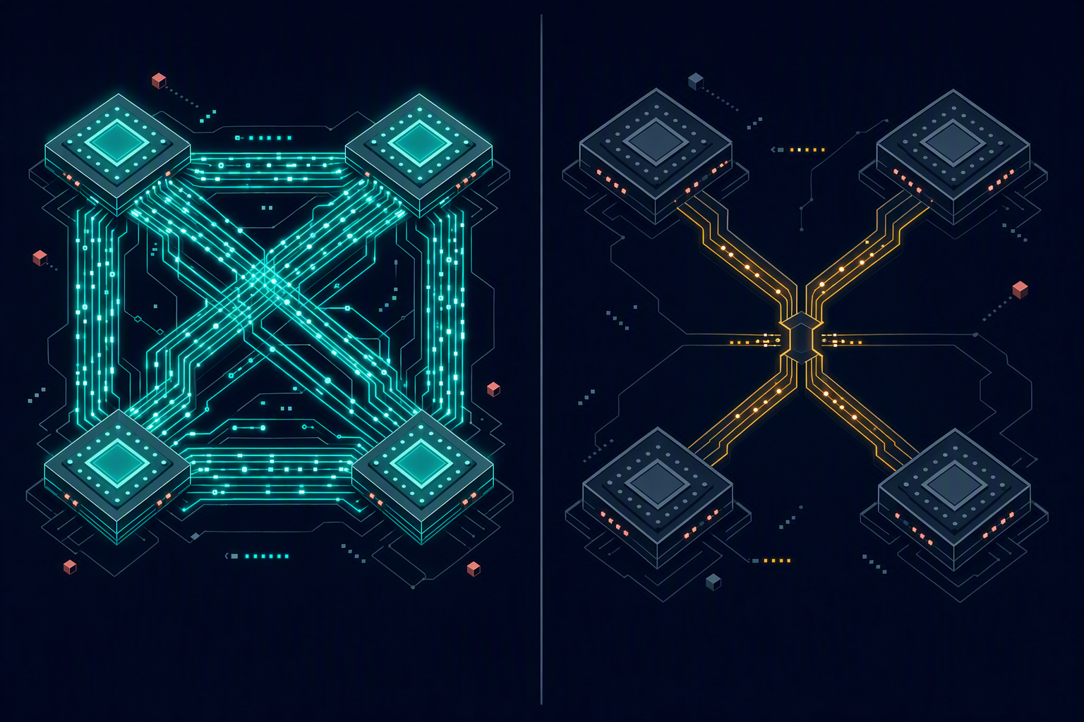
Figure 1.4.2 — Same four GPUs, same model, same launch command. Topology — not GPU count — decides whether tensor parallelism helps you or taxes you.

---

The mechanism

Three collectives, distinguished by ownership

Do not memorise names. Ask two questions: what does each rank own before, and what after? The reduction operator — usually sum — sits between those two states.

Collective	Before, per rank	After, per rank	Used in TP for
All-gather	one shard	the concatenation of all \(N\) shards	Reassembling a column-sharded activation
Reduce-scatter	a full-size partial	one shard of the elementwise sum	Row-sharded output when the next op is also sharded
All-reduce	a full-size partial	the complete elementwise sum	Row-sharded output when the next op needs the whole tensor

Concretely, with two ranks holding [1,2,3,4] and [10,20,30,40]: all-gather gives both [1,2,3,4,10,20,30,40]. Reduce-scatter sums to [11,22,33,44] and leaves rank 0 with [11,22], rank 1 with [33,44]. All-reduce leaves both with the full [11,22,33,44] — which exposes the identity that explains its cost:

flowchart LR
    A["Full partial<br/>on every rank"] --> RS["Reduce-scatter<br/>(sum, then split)"]
    RS --> B["One reduced shard<br/>per rank"]
    B --> AG["All-gather<br/>(collect, no arithmetic)"]
    AG --> C["Full reduced tensor<br/>on every rank"]
    A -.->|"equivalent to"| C

Figure 1.4.3 — All-reduce is two ownership changes bolted together. Every byte of payload therefore crosses the fabric twice, which is where the factor of 2 in the cost model comes from.

The cost model, derived

Start with a single point-to-point message of \(S\) bytes:

\[ T(S) \;\approx\; \alpha \;+\; \frac{S}{\mathrm{BW}} \tag{1.4.1} \]

\(\alpha\) is the fixed per-hop cost — kernel launch, rendezvous, synchronisation — paid even for a zero-byte message. \(\mathrm{BW}\) is sustained link bandwidth.

Now the ring. The tensor is cut into \(N\) chunks. Reduce-scatter runs \(N-1\) steps, each rank forwarding one chunk of \(S/N\) bytes to its neighbour and accumulating what arrives; all-gather runs another \(N-1\) steps circulating the finished chunks. So each rank sends

\[ \underbrace{(N-1)\frac{S}{N}}_{\text{reduce-scatter}} \;+\; \underbrace{(N-1)\frac{S}{N}}_{\text{all-gather}} \;=\; \frac{2S(N-1)}{N} \ \text{bytes over } 2(N-1) \text{ steps}, \tag{1.4.2} \]

and the time is the sum of the two costs across all those steps:

\[ T_{\text{ring}}(S, N) \;\approx\; \underbrace{2(N-1)\,\alpha}_{\text{latency term}} \;+\; \underbrace{\frac{2(N-1)}{N}\cdot\frac{S}{\mathrm{BW}}}_{\text{bandwidth term}} \tag{1.4.3} \]

Two regimes fall straight out. Set the terms equal and solve for the message size at which they balance:

\[ S^{*} \;=\; N \cdot \alpha \cdot \mathrm{BW} \tag{1.4.4} \]

Below \(S^{*}\) you are in the latency regime: the collective's duration is set by step count, and link bandwidth is nearly irrelevant. Above it you are in the bandwidth regime: step count barely matters and the fabric's width is everything.

Figure 1.4.4 — Below the crossover, you are paying for the fittings and not the fluid. Above it, the pipe's width is the only thing that matters. The same API call lives in both worlds.

Worked example — where the crossover sits

Take \(N = 2\), a per-hop \(\alpha \approx 5\ \mu s\), and an achievable NVLink bandwidth of ≈ 250 GB/s:

\[S^{*} = 2 \times 5\times10^{-6} \times 250\times10^{9} \approx \mathbf{2.5\ MB}.\]

Every collective smaller than about 2.5 MB is a latency problem, not a bandwidth problem. Hold that number; tensor-parallel decode never comes close to it.

These \(\alpha\) and bandwidth values are order-of-magnitude figures used to instantiate the model. This chapter has no committed NCCL measurement — the artifact in code/M1T4-multi-gpu-plumbing/ exists to produce one on real hardware. Treat every curve here as a model.

The payoff: TP=2 on Llama-3.1-8B

A tensor-parallel decoder block shards attention and the MLP the same way: the first matrix is split by columns (no communication — each rank produces its own slice of the intermediate), the second by rows, so each rank produces a full-width partial that must be summed. That is one all-reduce after the attention output projection and one after the MLP down projection. With \(L = 32\) layers:

\[ n_{\text{coll}} = 2L = \mathbf{64\ \text{all-reduces per token}} \tag{1.4.5} \]

Each one carries the residual-stream activation for the whole batch:

\[ S_{\text{TP}} \;=\; B \cdot d \cdot s \tag{1.4.6} \]

Worked example — how big is a decode collective, really?

At \(B = 1\), \(d = 4096\), \(s = 2\) (bf16):

\[S_{\text{TP}} = 1 \times 4096 \times 2 = 8{,}192\ \text{bytes} = \mathbf{8\ KiB}.\]

Eight kilobytes. Against a crossover of 2.5 MB, that is three hundred times too small to touch the bandwidth term. Even at \(B = 64\) it is 512 KiB — still latency-dominated.

Conclusion: tensor-parallel decode never uses your interconnect's bandwidth. It uses its latency. A 600 GB/s fabric and a 64 GB/s one are, for this workload, separated almost entirely by their \(\alpha\) — NVLink wins because direct peer-to-peer copies have a far lower fixed cost than transfers staged through a host bridge, not because they are wider.

So what does TP=2 buy? Decode is bandwidth-bound on HBM, so halving the weights halves the dominant term:

Quantity	TP=1	TP=2
Weight bytes read per GPU per token	16.06 GB	8.03 GB
Weight-read time at 1.5 TB/s	10.7 ms	5.35 ms
Collective tax (\(64 \times \alpha_{\text{eff}}\)), NVLink at \(\alpha_{\text{eff}} \approx 5\ \mu s\)	0	0.32 ms
Step time (model)	10.7 ms	5.67 ms
Speedup	1.00×	1.89×

Real, and sublinear. You never get 2×, because the tax is fixed while the saving shrinks with every GPU you add. Note that the ring formula's \(2(N-1)\alpha\) overstates the \(N=2\) case — NCCL does not build a ring for two ranks on small messages, it uses a direct peer copy with its low-latency protocol. Use Equation 1.4.3 to understand scaling; use a benchmark to get a number.

Now invert it. How slow must the fabric be before TP=2 is a loss? Break-even is when the collective tax equals the saved weight-read time:

\[ 2L\,\alpha^{*} \;=\; \frac{M_w}{2\,B_{mem}} \qquad\Longrightarrow\qquad \alpha^{*} \;=\; \frac{M_w}{4\,L\,B_{mem}} \tag{1.4.7} \]

Worked example — the break-even latency

\(M_w = 16.06\times10^{9}\) bytes, \(L = 32\), \(B_{mem} = 1.5\times10^{12}\) byte/s:

\[\alpha^{*} = \frac{16.06\times10^{9}}{4 \times 32 \times 1.5\times10^{12}} \approx \mathbf{84\ \mu s}.\]

If one small all-reduce costs more than ~84 µs, TP=2 makes Llama-3.1-8B decode slower than a single GPU. NVLink, at single-digit microseconds, has an order of magnitude of headroom. PCIe with working peer-to-peer, in the tens of microseconds, is uncomfortable but usually still ahead. PCIe with P2P unavailable — every transfer staged through pinned host memory — under contention is exactly where you cross 84 µs and pay double for a slowdown.

Two effects push the real crossover lower still: two half-size GEMMs are less efficient than one full-size GEMM, and the collective is a hard barrier, so the slowest rank sets the pace.

Figure 1.4.5 — No single seam is expensive. There are sixty-four of them per token, and they add up to the entire margin between a win and a loss.

Prefill lives in the other regime

Swap decode for prefill and every conclusion inverts. Prefill processes \(T_{in}\) tokens at once, so Equation 1.4.6 becomes \(S = T_{in} \cdot d \cdot s\).

Worked example — the same collective, one thousand times larger

A 4,096-token prompt: \(S = 4096 \times 4096 \times 2 = 33.6\) MB — past the 2.5 MB crossover, so the bandwidth term now rules. At \(N = 2\) the ring factor \(2(N-1)/N = 1\), so each rank moves the full 33.6 MB:

Fabric	Effective BW (model)	Per collective	× 64 per prefill
NVLink 3.0	≈ 250 GB/s	134 µs	8.6 ms
PCIe Gen4 ×16	≈ 24 GB/s	1.40 ms	90 ms

A 10× topology gap becomes a 10× TTFT gap — 81 ms of extra wall clock on the PCIe box, per request, invisible in any decode benchmark you ran first.

So a single "interconnect bandwidth" number never answers the question. Decode asks your fabric about latency; prefill asks about bandwidth. A machine can be fine at one and terrible at the other.

Read the box before you trust the flag

Run nvidia-smi topo -m on any unfamiliar machine first. It prints a matrix of pairwise paths; the codes are the whole story:

Code	Meaning	Consequence for TP
NV12	12 NVLink links to that peer — the full 600 GB/s	Best case. TP=2 across this pair is straightforward
NV4	4 NVLink links — ≈ 200 GB/s	Common in hybrid-mesh 8-GPU nodes. Fine, but pin your TP pairs deliberately
PIX / PXB	PCIe, through one or more switches, no host bridge	P2P usually works; latency higher than NVLink
PHB	Traverses the CPU's PCIe host bridge	P2P often unavailable; transfers may stage through host memory
SYS	Crosses the inter-socket link (UPI/xGMI)	Worst path in the box. Never put a TP group across it

flowchart TD
    T["nvidia-smi topo -m"] --> Q{"Path between the<br/>ranks you intend to pair?"}
    Q -->|"NV12 / NV4"| A["Direct NVLink.<br/>Latency ~ single-digit µs.<br/>TP=2 or 4 is viable"]
    Q -->|"PIX / PXB"| Bx["PCIe with P2P.<br/>Tens of µs.<br/>Benchmark before committing"]
    Q -->|"PHB / SYS"| C["Host bridge or cross-socket.<br/>Re-pin ranks, or do not use TP<br/>for latency at all"]
    A --> D{"Does the model fit<br/>on one GPU?"}
    Bx --> D
    C --> E["Use TP only to fit the model.<br/>Expect a latency cost, not a win"]
    D -->|"Yes"| F["TP is optional.<br/>Measure TP=1 vs TP=2 on<br/>your own traffic before enabling"]
    D -->|"No"| G["TP is mandatory.<br/>Use the smallest N that fits"]

Figure 1.4.6 — The decision procedure. Note that the topology check comes first: it can veto the whole idea before model size is even relevant.

The codes tell you what the hardware can do, not what NCCL chose. NCCL_DEBUG=INFO with NCCL_DEBUG_SUBSYS=INIT,GRAPH,COLL prints the graph it actually built — for diagnosis only.

Algorithm bandwidth is not bus bandwidth

One definitional trap, because it silently corrupts every comparison you make. If a 1 GiB all-reduce completes in 1 second, the algorithm bandwidth is 1.07 GB/s — payload divided by time. But Equation 1.4.2 says the fabric carried \(2(N-1)/N\) times that. nccl-tests reports the corrected figure, bus bandwidth:

\[ \mathrm{BW}_{\text{bus}} \;=\; \mathrm{BW}_{\text{alg}} \cdot \frac{2(N-1)}{N} \tag{1.4.8} \]

At \(N = 4\) the factor is 1.5, so 100 GB/s algorithmic is 150 GB/s bus. Only the bus figure is comparable to a link's physical peak — so label which definition every number uses, every time.

Four ways to publish a wrong interconnect number

Benchmarking without warmup. The first collective pays CUDA context setup, NCCL bootstrap, buffer registration, and a cold clock ramp — tens of times slower than steady state. Warm up, then report medians and percentiles.

Assuming NVLink exists. Cloud instance types and rack builds of the same GPU differ. A cost model built on an assumed fabric is a fabricated cost model.

Measuring bandwidth with tiny messages. An 8 KiB all-reduce reports terrible GB/s because it measures \(\alpha\), not \(\mathrm{BW}\). That is not a slow fabric; that is the wrong question.

Comparing algorithm bandwidth against a link's peak. You will "discover" 30% efficiency that is really 90%, and tune a system that was already fine.

On newer silicon

NVLink 4 (Hopper) reaches 900 GB/s per GPU and NVLink 5 (Blackwell) 1.8 TB/s, and NVSwitch turns a node into a uniform all-to-all domain where every pair gets full bandwidth instead of the ragged NV4/PHB mixture a direct-attach mesh gives you. All of it compresses \(\alpha\) and widens \(\mathrm{BW}\), moving Equation 1.4.7's break-even firmly in TP's favour.

We cannot test any of it here. The baseline is A100 SXM (SM 8.0) with NVLink 3.0, TP widths of 1, 2, and 4 only, and multi-node behaviour simulated rather than run. Read the vendor numbers as a direction of travel, not as something you have verified.

---

In practice

Run nvidia-smi topo -m before anything else. Two seconds, and it decides whether the rest of the exercise is worthwhile. Archive it beside any benchmark you keep; a bandwidth graph without a topology snapshot is not reproducible evidence.

Pick the TP degree from constraints, not ambition. In vLLM, --tensor-parallel-size must divide the head counts — Llama-3.1-8B has 32 attention heads and 8 KV heads, so TP ∈ {1, 2, 4, 8}. This curriculum uses 1, 2, and 4, and simulates multi-node. Use the smallest degree that fits the model; anything beyond that must earn its collective cost on your own traffic.

Launch one process per GPU and bind it before CUDA initialises. Inside containers, visible-device indices are local aliases — physical GPU 5 is cuda:0 to the process that owns it — and confusing the two routes collectives across the worst link in the box.

Sweep 1 KiB to hundreds of MiB. The left end measures \(\alpha\), the right end \(\mathrm{BW}\), and the knee between them is the only informative part of the curve.

---

Failure modes

Symptom	Cause	Fix
TP=2 is slower than TP=1 on the same model	Collective tax exceeds saved weight-read time — Equation 1.4.7 crossed	Check topology first. If PHB/SYS, re-pin ranks. If genuinely PCIe-only, use TP only to fit the model
Decode scales poorly but prefill scales fine	Decode is latency-bound at 8 KiB messages; prefill is bandwidth-bound at tens of MB	Different regimes, different fixes. Attack \(\alpha\) (P2P, fewer collectives, CUDA graphs) for decode, not bandwidth
Bandwidth is flat and poor at every message size	P2P disabled, wrong process/GPU affinity, or traffic crossing a host bridge	nvidia-smi topo -m, then NCCL_DEBUG=INFO NCCL_DEBUG_SUBSYS=INIT,GRAPH to see the graph NCCL built
First measurement is 10–50× slower than the rest	No warmup: bootstrap, buffer registration, clock ramp	Discard warmup iterations explicitly; report medians and p99, never means
Reported bandwidth "exceeds" the link, or looks absurdly low	Algorithm bandwidth compared against physical peak, or vice versa	Apply Equation 1.4.8 and label which definition every number uses
Job hangs at startup with no error	Ranks disagree on world size or rendezvous, or one rank died silently	Check every rank's log, not rank 0's. Run a minimal 4-byte all-reduce before loading model code
Throughput is fine, tail latency is terrible	One rank is slower (thermal, MIG neighbour, different clocks) and the barrier propagates it	Collectives run at the speed of the slowest rank. Check per-GPU clocks and utilisation, not the aggregate

---

Do it

Run the NCCL all-reduce artifact on a 2-GPU host, then a 4-GPU host if you have one:

WORLD_SIZE=2 ./run.sh

It sweeps 1 KiB → 512 MiB twice — once on NCCL's normal route, once with NCCL_P2P_DISABLE=1 as a controlled degradation run — and writes both curves as JSON plus a combined plot, recording algorithm and bus bandwidth side by side so you cannot conflate them. It refuses to synthesise a curve it did not measure, and the second mode is a comparison, not a claim that every byte took a specific physical route.

Success criterion, all relative and explanatory:

1. You can point at the knee in each curve, state its message size, and check it against Equation 1.4.4 solved for the \(\alpha\) your machine actually has.
2. You can explain the large-message gap between the two modes from your captured nvidia-smi topo -m.
3. Using your measured small-message \(\alpha\), you can predict via Equation 1.4.7 whether TP=2 wins or loses on Llama-3.1-8B decode before launching a serving engine — then launch one and check.

That snapshot is also the input to the collective extension in LAB-M1.

---

Summary

• Tensor parallelism halves the weight bytes each GPU reads and adds \(2L\) all-reduces per token. Only the first effect is guaranteed to help.
• \(T_{\text{ring}} \approx 2(N-1)\alpha + \frac{2(N-1)}{N}\frac{S}{\mathrm{BW}}\). Below \(S^{*} = N\alpha\,\mathrm{BW}\) a collective is a latency problem; above it, a bandwidth problem.
• Llama-3.1-8B decode collectives are 8 KiB at batch 1 — three orders of magnitude inside the latency regime. Prefill collectives at 4 K context are 33.6 MB, firmly in the bandwidth regime. Same model, opposite constraints.
• The model breaks even at \(\alpha^{*} \approx 84\ \mu s\) per collective. NVLink has an order of magnitude of headroom; a host-staged PCIe path under contention does not.
• All-reduce = reduce-scatter + all-gather, so every byte crosses the fabric twice — which is why bus bandwidth is algorithm bandwidth times \(2(N-1)/N\).

Key terms

all-reduce · NVLink · rank · tensor parallelism · bandwidth-bound

---

Exercises

Recall

1. State what each rank owns before and after all-gather, reduce-scatter, and all-reduce. Which two compose into the third?
2. Why is nvidia-smi topo -m the first command you run on an unfamiliar multi-GPU box? What do NV4 and SYS each imply for a TP=2 decision?

Derive

1. For ring all-reduce at \(N = 4\), how many bytes does each rank send relative to the tensor size, and over how many steps? Convert an algorithm bandwidth of 120 GB/s into bus bandwidth.
2. A model has \(L = 40\) layers, \(d = 5120\), bf16. Compute the per-collective message size for TP decode at \(B = 1\) and at \(B = 128\), and the number of collectives per token. Using \(\alpha = 6\ \mu s\) and \(\mathrm{BW} = 250\) GB/s, state which regime each case is in.

Design

1. You serve Llama-3.1-8B on a 4-GPU node. nvidia-smi topo -m reports NV12 between GPUs 0–1 and 2–3, and SYS between the two pairs. Traffic is 6 K-token prompts, 300-token responses, and you are TTFT-sensitive. Choose a parallelism configuration and defend it. What would change your answer?

Worked solutions

**1.** *All-gather*: before, each rank owns one distinct shard; after, every rank owns the ordered concatenation of all $N$ shards — no arithmetic occurs. *Reduce-scatter*: before, a full-size partial each; after, one shard of the elementwise sum. *All-reduce*: before, a full-size partial each; after, the complete sum everywhere. **Reduce-scatter followed by all-gather equals all-reduce** (Figure 1.4.3), which is why each rank moves $2S(N-1)/N$ bytes rather than $S(N-1)/N$. **2.** Because topology can veto the whole plan before model size is relevant, and because two machines with identical `nvidia-smi -L` output can differ by ~10× on the number that decides it (600 GB/s NVLink vs 64 GB/s PCIe Gen4 ×16). `NV4` = four NVLink links ≈ 200 GB/s direct — good, but pin your TP pairs deliberately, since other pairs in the node may be worse. `SYS` = the path crosses the inter-socket link: the worst route in the box, P2P typically unavailable, and a TP group must never straddle it. **3.** From Equation 1.4.2, each rank sends $2S(N-1)/N = 2S(3)/4 = 1.5S$ bytes, over $2(N-1) = 6$ steps. Bus bandwidth (Equation 1.4.8) $= 120 \times 1.5 = \mathbf{180\ \text{GB/s}}$. **4.** Collectives per token $= 2L = \mathbf{80}$. Message size $= B \cdot d \cdot s$: at $B=1$, $1 \times 5120 \times 2 = \mathbf{10\ KiB}$; at $B=128$, $128 \times 5120 \times 2 = 1{,}310{,}720$ bytes $= \mathbf{1.25\ MiB}$. Crossover (Equation 1.4.4) at $N=2$: $S^{*} = 2 \times 6\times10^{-6} \times 250\times10^{9} = 3.0$ MB. So **both cases are latency-dominated** — $B = 128$ sits at roughly 44% of the crossover. The practical reading: raising batch size does not move TP decode out of the latency regime, it amortises the same fixed tax over more tokens. A throughput win, not a latency one. **5.** **Run TP=2 within each NVLink pair, and data-parallel across the two pairs** — two independent replicas, each on `NV12`. Never TP=4: it forces every all-reduce across the `SYS` link, and a ring at $N=4$ takes $2(N-1) = 6$ steps, at least two of which traverse the worst path in the machine. TTFT sensitivity makes this decisive. At 6 K prompts each prefill collective is $6144 \times 4096 \times 2 = 50.3$ MB — deep in the bandwidth regime, exactly where the `SYS` path would eat your TTFT. And at 14.96 GiB the model fits on one A100 four times over, so TP is buying latency, not feasibility. TP=1 with four replicas is a legitimate answer here and should be your measured baseline. Two things change it. **A bigger model**: if it no longer fits in two GPUs, TP=4 is mandatory and the `SYS` cost is the price of running at all. **A throughput-first SLO**: two TP=2 replicas win even more clearly, since you get twice the batch capacity with zero cross-pair traffic.

---

Going deeper

• NCCL user guide — collective operations — the authoritative definitions of the three ownership changes
• NVIDIA NCCL Tests — read src/all_reduce.cu and the bus-bandwidth derivation in the README before trusting any number you produce
• Megatron-LM: Efficient Large-Scale Language Model Training on GPU Clusters — §3 is where the "two all-reduces per layer" sharding comes from
• PyTorch distributed communication package — the API surface the artifact uses
• NVIDIA A100 architecture whitepaper — the NVLink 3.0 link counts and per-link rates quoted here

---

Next: Chapter 1.5 — Toolchain Diagnostics, where reading the machine becomes a repeatable procedure rather than a lucky guess.