T2.1 — Anatomy of a Decoder Block

In one line: A decoder block repeatedly reads a residual stream, mixes information with attention and an MLP, then writes updates back into that same stream.

Skill	00-foundations
Module	M2 — Transformer Internals from the Inference Angle
Audience	New graduate engineer
Time	~110 min
Prereqs	M1; matrix multiplication and tensor shapes
Status	built

Why this matters

Model names hide the tensors that determine VRAM, FLOPs, and serving behavior. If you can turn a decoder configuration into projection shapes and parameter counts, you can estimate weight memory before downloading a checkpoint and recognize which architectural changes affect inference cost.

The mental model

Imagine a sentence represented as a row of vectors. Each vector is a token’s current working representation. A decoder block does not replace those vectors with a completely new object. It computes two updates—one from attention and one from an MLP—and adds both updates back to the existing vectors. That continuing workspace is the residual stream.

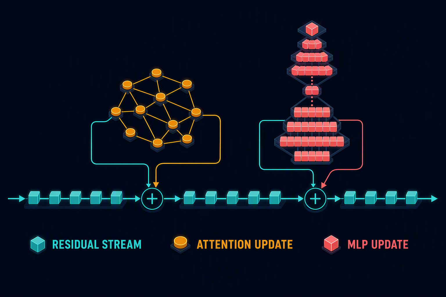
Attention and the MLP add updates while the residual stream preserves a continuous path.

The block is therefore easier to understand as a loop than as a collection of fashionable layer names:

flowchart LR
    X[Residual stream<br/>B × T × d] --> N1[RMSNorm]
    N1 --> A[Self-attention]
    A --> R1[Add to residual]
    X --> R1
    R1 --> N2[RMSNorm]
    N2 --> M[Gated MLP]
    M --> R2[Add to residual]
    R1 --> R2

Attention mixes information across token positions; the MLP transforms each position independently; residual additions preserve a stable path through all layers.

Here B is batch size, T is the number of token positions processed together, and d is hidden size. The overall tensor shape remains B × T × d across the block even though attention temporarily separates the final dimension into heads and the MLP temporarily expands it.

The mechanism

From token IDs to the residual stream

The model first looks up each integer token ID in an embedding table with shape vocab_size × d. If the vocabulary contains 32,000 entries and d=4096, the table contains about 131 million parameters. The lookup produces one length-4096 vector per token. Position information is then introduced—often inside attention through RoPE rather than by adding a learned position vector.

RMSNorm rescales each token vector according to its root-mean-square magnitude. For a vector \(x\in\mathbb{R}^d\), a simplified form is

\[ \operatorname{RMSNorm}(x)=g\odot\frac{x}{\sqrt{\frac{1}{d}\sum_i x_i^2+\epsilon}}, \]

where g is a learned length-d scale. Unlike LayerNorm, RMSNorm does not subtract the mean. Its parameter count is tiny compared with the projection matrices, but its memory reads and kernel launches still appear in latency profiles.

Attention changes who can influence whom

Self-attention creates queries, keys, and values from the normalized residual stream. With ordinary multi-head attention, the three projection matrices are each approximately d × d. Attention compares each query with keys from allowed earlier positions, uses softmax to turn scores into weights, combines the values, and applies an output projection of shape d × d.

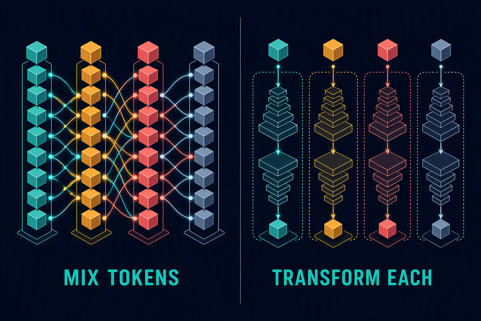
Attention mixes positions; the MLP transforms each position independently.

Causal masking prevents position t from reading positions after t. During training or prefill, the model can compute many positions in parallel because the mask enforces causality mathematically. During generation, the token at position t+1 does not exist until position t has produced it, so decode remains sequential across output steps.

With grouped-query attention, query heads still span the full hidden size, but fewer key and value heads are projected. If d=4096, there are 32 query heads, and each head has dimension 128, then eight KV heads occupy 8×128=1024 output features. Each K and V matrix becomes 4096×1024 rather than 4096×4096. This reduces attention parameters and, more importantly, the KV-cache size introduced in T2.2.

The MLP changes each token independently

After the attention update is added to the residual stream, the block normalizes again and applies an MLP separately to every token position. A common gated MLP has three matrices:

\[ \operatorname{MLP}(x)=W_{down}\left(\operatorname{SiLU}(W_{gate}x)\odot W_{up}x\right). \]

Both gate and up expand from d to d_ff, while down contracts from d_ff to d. The parameter count is therefore approximately 3 × d × d_ff. For d=4096 and d_ff=11008, one layer’s MLP contains roughly 135 million weights. Across 32 layers, that is about 4.33 billion parameters—larger than the attention share in the accompanying 6.74B educational configuration.

This is a useful correction to the phrase “attention model.” In many dense decoders, the MLP owns most parameters and much of the arithmetic. Attention is special because its work and cache depend on sequence length; the MLP is large because of its projection matrices.

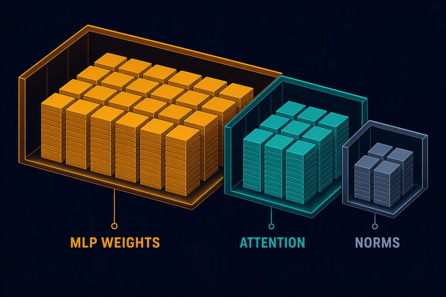
The MLP often owns more weights even though attention defines token interaction.

Deriving the familiar parameter estimate

For simple multi-head attention, Q, K, V, and output projections contribute roughly 4d² parameters per layer. A classic non-gated MLP with intermediate size 4d contributes 2 × d × 4d = 8d². Together they give

\[ \text{parameters}\approx L(4d^2+8d^2)=12Ld^2. \]

This rule is a rough mental estimate, not a universal formula. Gated MLPs use three matrices; modern intermediate sizes are not always 4d; GQA shrinks K and V; embeddings and the language-model head can be large; MoE changes the calculation completely. The point of the rule is to estimate the scale before performing an exact count.

The code artifact reads these choices from a configuration. On its educational dense configuration it estimates 6.74B parameters: 4.33B in MLPs, 2.15B in attention, and about 262M across embeddings and the untied output head. Its educational GQA configuration has a larger MLP and vocabulary but only 1.34B attention parameters because K and V use eight heads.

In practice

When opening an unfamiliar config.json, locate these fields first: hidden_size, intermediate_size, num_hidden_layers, num_attention_heads, num_key_value_heads, vocab_size, and tie_word_embeddings. Compute head_dim = hidden_size / num_attention_heads and verify it is integral. Then write the actual projection shapes before trusting a model-size label.

Parameter count converts to raw weight bytes by multiplying by storage bytes per parameter. A 7.5B-parameter model needs about 15 GB for bf16 weights before runtime overhead. Four-bit storage suggests 3.75 GB before scales, alignment, and other tensors. This is not the total serving VRAM budget; KV cache, activations, CUDA context, workspaces, and fragmentation come later.

Configuration names vary among model families, and some architectures add biases, shared experts, convolution, low-rank projections, or separate embedding dimensions. Treat the counter as an inspectable baseline. Verification means comparing its categories with the checkpoint’s actual tensor names and shapes, not merely matching a rounded model-card label.

Failure modes

Symptom	Cause	Fix
Estimate is off by hundreds of millions	Embedding and LM head tying was assumed incorrectly, or vocabulary is large	Inspect tie_word_embeddings and checkpoint tensor identities
Attention count is too high	The model uses GQA/MQA but the counter assumed one KV head per query head	Read num_key_value_heads and derive K/V output width
MLP count is wrong	The architecture is gated, uses a different intermediate size, or is MoE	Count the named projection matrices and use the configured intermediate_size
Hidden size does not divide by query heads	The config was mapped incorrectly or uses a nonstandard head dimension field	Stop and inspect model source instead of silently rounding
Raw weight bytes fit but loading OOMs	Runtime memory is not only parameters	Add context, workspaces, cache, activations, and allocator headroom

Do it

Run the parameter counter. Predict the largest category for each bundled educational configuration before viewing the JSON. Then point it at a real model configuration and verify the estimate against checkpoint tensor shapes.

Success requires explaining every projection shape and bringing the total within 1% of the tensors you intentionally cover. Any excluded tensors must be named rather than hidden inside the error percentage.

Check

1. Why does the residual stream retain shape B × T × d even though the MLP expands to d_ff?
2. For d=4096, 32 query heads, and eight KV heads, what are head_dim and the K projection’s output width?
3. Why is 12Ld² a useful estimate but an unsafe exact formula for a modern decoder?

Going deeper

• Attention Is All You Need
• Root Mean Square Layer Normalization
• LLaMA: Open and Efficient Foundation Language Models
• Hugging Face Transformers — Llama model source