Chapter 2.2 — Attention and the KV Cache¶
In one line: The KV cache is the thing you are actually selling — weights are a fixed cost you pay once, but cache is the per-customer inventory that decides how many users fit on a GPU.
| Part | II — The Model |
| Chapter | 2.2 |
| Time | ~120 min |
| Prereqs | 1.1 Memory hierarchy, 2.1 Decoder block anatomy |
| Notation | \(L\), \(B\), \(T\), \(H_{kv}\), \(d_h\), \(s\) |
| Status | reviewed |
Where we are
Chapter 2.1 established that a decoder block reads a residual stream and adds two updates back into it. This chapter opens the attention half of that block and finds the single largest memory consumer in production LLM serving. Everything in 2.3 (head sharing), 2.4 (prefill vs decode), and the whole of Part III is downstream of the one formula derived here.
Why this matters¶
Here is the uncomfortable arithmetic that runs every inference business.
You rent an A100 80 GB. Llama-3.1-8B in bf16 occupies 14.96 GiB of it. That number never changes — not with traffic, not with time of day, not with how many customers you have. It is rent.
Everything else on that card, roughly 62 GiB after the CUDA context and activation headroom, exists to hold KV cache. And KV cache is consumed per token, per user. At Llama-3.1-8B's dimensions, one cached token costs 128 KiB. So your 62 GiB buys about 496,000 tokens of live context — and not one token more.
That single number is your capacity. Sixty users at 8 K context each, or fifteen users at 32 K, or one user at 131 K with three-quarters of the card idle. The model is identical in all three cases. The revenue is not.
The sentence to remember
Weights determine whether the model fits. KV cache determines how many customers fit with it. Almost every capacity decision in this curriculum is a KV cache decision wearing a disguise.
The mental model¶
Attention is a lookup over notes left behind by earlier tokens.
Every token, as it is processed, writes two things into a shared ledger: a key, which advertises what kind of information I can offer, and a value, which is the information itself. When a new token arrives it forms a query — what kind of information I am looking for — compares that query against every key in the ledger, and mixes the matching values into its own representation.
The crucial property is that the ledger is append-only. Token 500's key and value are computed from token 500's input and the model's weights. Neither changes when token 501 arrives, or token 5,000. Recomputing them at every step would be recomputing a constant.
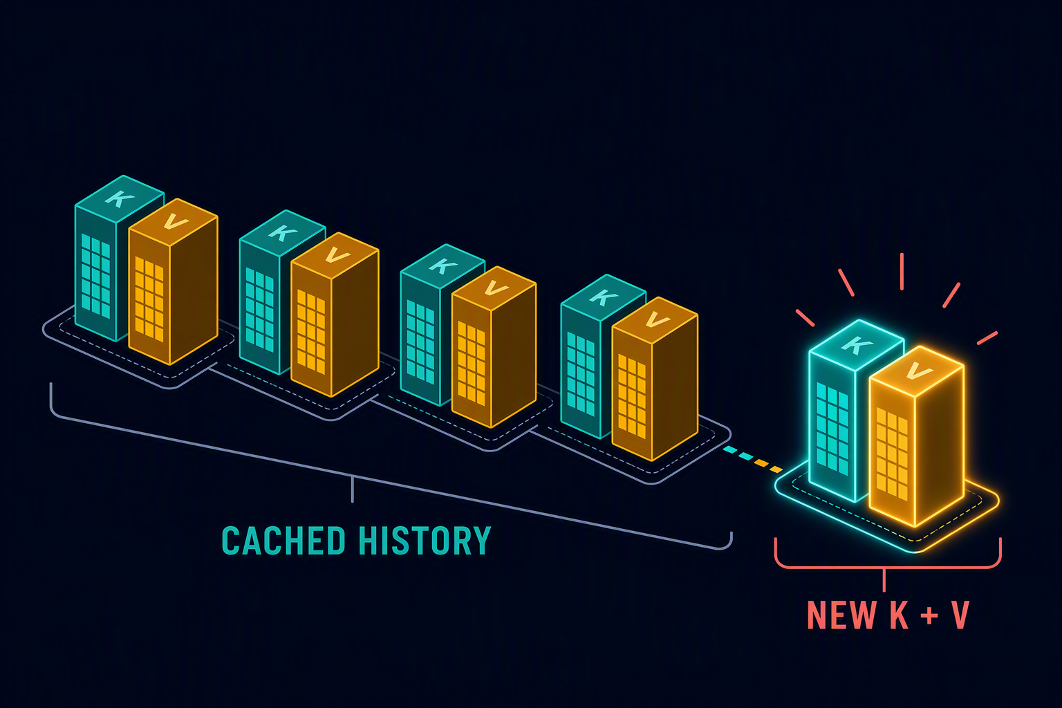
Figure 2.2.1 — Each generated token appends exactly one key/value pair per layer, forever. The stack only grows; nothing already in it is ever revised.
So we keep the ledger. That is the entire idea. The consequences are what take the rest of the chapter.
The mechanism¶
The asymmetry between Q and K, V¶
Students reliably ask the same excellent question: if we cache K and V, why not cache Q too?
The answer is a real asymmetry in how the three tensors are consumed, and it is worth being precise about, because it is the load-bearing insight of the chapter.
For a single head, the attention output at position \(t\) is
Read the subscripts carefully. Position \(t\) uses one query — its own — against all keys and values from positions \(1\) through \(t\). Now ask what position \(t+1\) needs: it needs \(q_{t+1}\), which does not exist yet, and \(K_{1:t+1}\), \(V_{1:t+1}\), which is the previous ledger plus one new pair.
\(q_t\) appears nowhere in that expression. Once token \(t\)'s output has been computed and passed up the stack, its query has done its entire job and is garbage. Keys and values, by contrast, are read by every future token for the rest of the sequence's life. A query is consumed once; a key and value are consumed forever. Cache the tensors with many future readers.
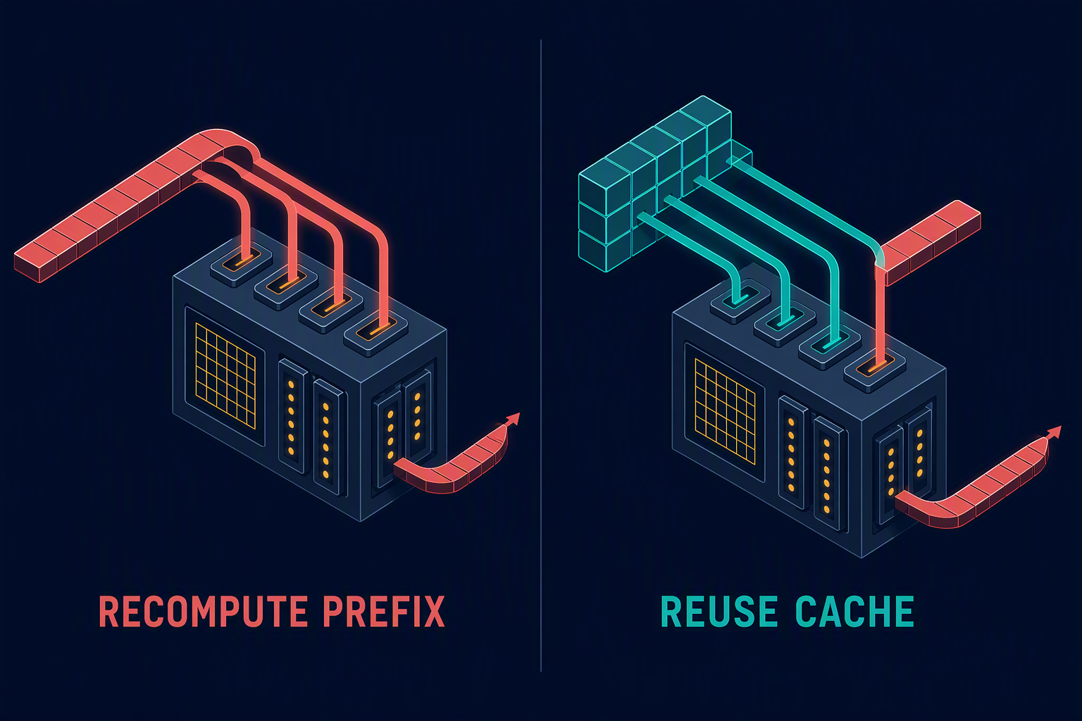
Figure 2.2.2 — Without a cache (left), step \(t\) re-projects the entire prefix. With a cache (right), step \(t\) projects exactly one token and reads what is already there.
Quantify what that saves. Generating \(T_{out}\) tokens without a cache means, at step \(t\), projecting \(t\) tokens through every layer — a total of \(\sum_{t=1}^{T_{out}} t \approx T_{out}^2/2\) token-projections. With a cache it is \(T_{out}\). For a 2,000-token response that is a 1,000× reduction in projection work. KV caching is not an optimisation. It is the difference between a product and a science experiment.
Deriving the size formula¶
Now the bill. Take it one dimension at a time and the formula assembles itself.
Start with a single key tensor, in a single layer, for a single sequence. Attention splits the hidden dimension into \(H_{kv}\) key/value heads of width \(d_h\), and there is one such vector per cached token:
Values have identical shape, which supplies a factor of 2. Every layer keeps its own independent cache, which supplies \(L\). Every concurrent sequence keeps its own, which supplies \(B\). Multiply:
Seven terms, each with a physical meaning, and each a lever someone will eventually try to pull:
| Term | Meaning | Can you change it? |
|---|---|---|
| \(2\) | K and V | No. It is two tensors |
| \(L\) | layers | Only by changing model |
| \(B\) | concurrent sequences | Yes — this is admission control |
| \(T\) | cached tokens per sequence | Yes — max_model_len, truncation, summarisation |
| \(H_{kv}\) | KV heads | Architecture — GQA/MQA/MLA, Chapter 2.3 |
| \(d_h\) | head dimension | Architecture |
| \(s\) | bytes per element | Yes — KV quantisation |
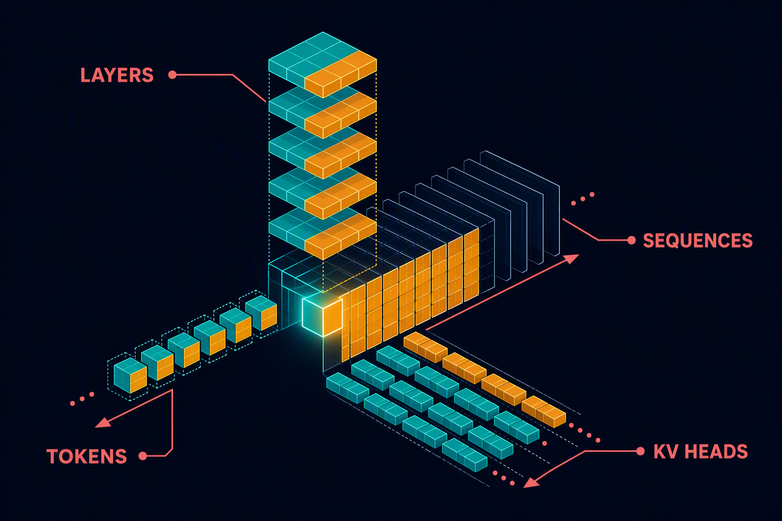
Figure 2.2.3 — Cache capacity is a product, not a sum. Halving any one dimension halves the whole thing; doubling two of them quadruples it.
Worked example — Llama-3.1-8B, one token
Substitute the running example's config: \(L = 32\), \(H_{kv} = 8\), \(d_h = 128\), \(s = 2\) (bf16), and set \(B = T = 1\) to get the per-token cost.
Memorise this. One Llama-3.1-8B token costs 128 KiB of cache. Everything else is then mental arithmetic: an 8 K conversation is \(8192 \times 128\ \text{KiB} = \mathbf{1\ GiB}\); a 128 K context is 16 GiB, more than the model's own weights, for a single user.
Two mistakes that will cost you a production incident
Using num_attention_heads instead of num_key_value_heads. Llama-3.1-8B reports 32 attention
heads and 8 KV heads. Use 32 and your estimate is 4× too large: you set concurrency limits
absurdly low and buy GPUs you did not need.
Dropping the leading factor of 2. Your estimate comes out at exactly half of what nvidia-smi
reports, and because it is off by such a clean factor you will spend an afternoon hunting a subtle
bug instead of a missing K-or-V.
The memory wall¶
Put the two numbers on one card and the shape of the business appears.
| Item | Bytes on an A100 80 GB |
|---|---|
| Model weights (bf16) | 14.96 GiB |
| CUDA context, fragmentation, activation headroom | ≈ 3 GiB |
| Remaining for KV cache | ≈ 62 GiB |
| Tokens that fit, at 128 KiB each | ≈ 496,000 |
Now spend it:
| Context per user | Concurrent users | Is the GPU doing useful work? |
|---|---|---|
| 2 K | 242 | Yes — the batch is fat and decode is efficient |
| 8 K | 60 | Yes |
| 32 K | 15 | Marginal |
| 128 K | 3 | No — you are renting an A100 to serve three people |
Nothing about the model changed across those rows. Only the workload did. This is why "which model should we serve?" is a less interesting question than "what is our context length distribution?" — and why the first thing to ask about any inference cost problem is for the length histogram.
Caching removes compute, not traffic¶
Here is the part that surprises people who have just learned to love the KV cache.
Caching eliminated the recomputation. It did not eliminate the reading. Equation 2.1 still requires \(q_t\) to be compared against all \(t\) keys and to mix all \(t\) values. Those bytes come out of HBM on every decode step, for every layer, for every sequence in the batch.
So a decode step reads two things: the model weights, once, shared across the whole batch; and the entire live KV cache, which is not shared at all, because every sequence reads its own.
Worked example — where the bandwidth actually goes
Sixty concurrent users, 8 K of context each, on one A100.
- Weight traffic per decode step: 14.96 GiB, read once and amortised across all 60 sequences
- KV traffic per decode step: \(60 \times 1\ \text{GiB} = \mathbf{60\ GiB}\)
- Total: ≈ 75 GiB per step
At a realistically achievable ~1.5 TB/s that is ≈ 54 ms per step. Sixty tokens emerge from it, so aggregate throughput is ≈ 1,100 tok/s and each user sees ≈ 18 tokens per second.
This is a back-of-envelope bound, not a benchmark — fused attention kernels and paged layouts beat parts of it. But the ratio is the lesson: 80% of the bytes moved were KV cache, not weights.
That ratio flips at a specific, computable point. KV traffic exceeds weight traffic when
which is about fifteen 8 K conversations. Below that line, quantising weights is the highest-leverage optimisation available to you. Above it, weight quantisation is rearranging deck chairs and you should be attacking the cache — GQA, KV quantisation, shorter contexts, prefix sharing. Teams routinely spend a quarter optimising the wrong side of that inequality.
Why engines page the cache¶
One more structural problem. A sequence's final length is unknown when it arrives. The naive allocator
therefore reserves max_model_len tokens up front — for Llama-3.1-8B with its 131 K window, that is
16 GiB reserved for a request that might produce forty tokens.
Reserve for the worst case and four users fit on the card. Reserve for the average and you crash the moment someone asks for an essay.
PagedAttention resolves this the way operating systems resolved it in 1962: allocate in small fixed blocks (typically 16 tokens), keep a block table per sequence mapping logical positions to physical blocks, and let the attention kernel follow that indirection. Blocks come from a shared pool and return to it the instant a sequence finishes. Waste falls from "an unused reservation" to "at most one partly-filled block per sequence" — under 1% instead of over 60%.
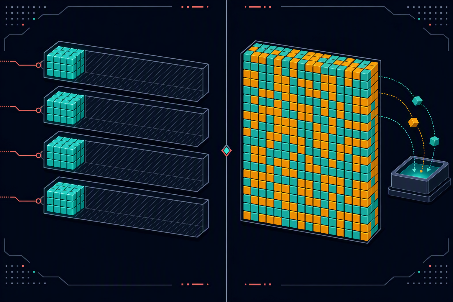
Figure 2.2.4 — The grey tail on the left is memory you paid for and never used. Paging converts it back into customers.
Paging changes placement, not volume. Equation 2.2 is untouched. That distinction matters when someone claims a serving engine "reduces KV cache": it reduces waste around the formula, and prefix sharing genuinely reduces \(B \cdot T\), but no scheduler ever makes a cached token cost less than 128 KiB.
In practice¶
The flags that map onto this chapter, using vLLM's names because they are the ones you will meet first:
| Flag | What it controls | How to reason about it |
|---|---|---|
--gpu-memory-utilization |
Fraction of the card the engine may claim (default 0.9) | Raising it buys KV blocks directly. Raise until fragmentation-related OOM appears under real traffic, then back off one step |
--max-model-len |
Per-sequence context ceiling | The single most effective capacity lever. Setting it to p99 prompt + p99 output rather than the model's maximum often doubles concurrency |
--block-size |
Tokens per KV block (default 16) | Larger blocks mean less metadata and more internal waste. Leave it alone unless profiling says otherwise |
--max-num-seqs |
Concurrency cap | Admission control. Without it, queueing degenerates into thrashing |
--kv-cache-dtype |
Cache element size \(s\) | Halving \(s\) halves Equation 2.2. Validate quality on long-context tasks, never on short ones |
--enable-prefix-caching |
Shares identical prompt prefixes across requests | A large win for shared system prompts and multi-turn chat; nothing at all for diverse one-shot traffic |
On newer silicon
FP8 KV cache (--kv-cache-dtype fp8_e5m2) requires SM 8.9+ — Ada, Hopper, Blackwell. On the A100
(SM 8.0) it either refuses to run or silently emulates, which is worse. The Ampere path is INT8 KV
cache, covered properly in Skill 03. Know that FP8 KV exists and why teams want it; do not put it in
a capacity plan for Ampere hardware.
Two operational habits are worth building now. First, always separate allocated blocks from used tokens on your dashboards — an engine can sit at 100% of its block pool while sequences are mostly short, which is a scheduling story, not a capacity story. Second, size for the aggregate live token count under your real length distribution, never for whether one maximum-length request fits alone. The single-request test passes happily on hardware that dies at 20 QPS.
Failure modes¶
| Symptom | Cause | Fix |
|---|---|---|
| Cached decode output diverges from full causal attention | Position, mask, append order, or head layout is wrong | Compare one token and one layer at a time; print tensor shapes at the append site. Divergence that grows with \(t\) is a mask bug; constant divergence is a layout bug |
| Estimate is exactly 4× the measured value | Used num_attention_heads on a GQA model |
Read num_key_value_heads from config.json |
| Estimate is exactly half the measured value | Dropped the leading factor of 2 | K and V |
| Fits in staging, OOMs at 20 QPS in production | Sized for one long request instead of aggregate live tokens | Size from the length histogram; set --max-num-seqs and --max-model-len from p99, not from the model card |
| Throughput collapses as contexts grow, despite caching | KV read traffic now dominates the decode step | Measure the bytes. Above ~122 K live tokens the cache, not the weights, owns your bandwidth — attack \(H_{kv}\), \(s\), or \(T\) |
| Cache appears to leak — utilisation climbs and never returns | Aborted or disconnected requests are not releasing blocks | Check the engine's preemption and cleanup metrics; confirm client cancellations actually propagate |
Do it¶
Run the raw KV-cache artifact. It implements causal attention twice — once over a whole sequence with a triangular mask, once one token at a time with an append-only cache — and asserts that the outputs match.
Success criterion. Two things, both objective:
- Cached and full-attention outputs agree to within
1e-5after you extend the artifact to multiple heads and layers. - You can predict the artifact's reported cache byte count before running it, from Equation 2.2 alone, exactly — not approximately.
The committed diagnostic shows a maximum difference of 8.64e-7 over 64 float32 tokens and a cache of
exactly 65,536 bytes. If your prediction and the printed number disagree, one of your seven terms is
wrong, and working out which one is the entire exercise.
Then do the arithmetic that matters commercially: take your own product's prompt and response length distribution and compute how many concurrent users fit on one A100. That number, not a benchmark, is what a capacity conversation is actually about.
Summary¶
- Attention needs every earlier token's keys and values; it never needs an earlier query. Cache the tensors with many future readers.
- \(M_{kv} = 2LBTH_{kv}d_hs\). Seven terms, four of which you can actually move.
- Llama-3.1-8B costs 128 KiB per cached token → 1 GiB per 8 K conversation → ≈ 496 K tokens fit on an A100 80 GB once the weights are in.
- Caching removes recomputation, not reading. Above roughly 122 K live tokens, KV traffic dominates weight traffic and your optimisation priorities invert.
- Paging fixes allocation waste, not the formula. No scheduler makes a token cheaper.
Key terms¶
KV cache · block · GQA · prefill · bandwidth-bound
Exercises¶
Recall
- State Equation 2.2 and define all seven terms with units.
- Why is an earlier token's query not needed at the next decode step, while its key and value are?
Derive
- A model has 24 layers, 4 KV heads, head dimension 128, and is served in bf16. Compute the bytes per cached token, then the cache for 4 concurrent 2,048-token sequences.
- You switch a 32-KV-head model to 8 KV heads and simultaneously quantise the cache from bf16 to int8. By what factor does capacity in tokens change, and what did you pay for it?
Design
- Your service runs Llama-3.1-8B on one A100 80 GB. Prompts average 6 K tokens with a shared 2 K-token system prefix; responses average 400 tokens. You currently serve 40 concurrent users and want 100 without adding hardware. Rank your levers by expected gain and name what each one costs you.
Worked solutions
**1.** $M_{kv} = 2LBTH_{kv}d_hs$ bytes. $2$ = one tensor each for K and V (dimensionless); $L$ = layers; $B$ = concurrent sequences; $T$ = cached tokens per sequence; $H_{kv}$ = key/value heads per layer; $d_h$ = elements per head; $s$ = bytes per element. **2.** In Equation 2.1, position $t$'s output uses $q_t$ against $K_{1:t}, V_{1:t}$. Position $t+1$ uses $q_{t+1}$ against $K_{1:t+1}, V_{1:t+1}$. The query index always equals the current position, so old queries never reappear; the key and value ranges are cumulative, so old keys and values reappear at every future step. **3.** Per token: $2 \times 24 \times 4 \times 128 \times 2 = 49{,}152$ bytes = 48 KiB. For $B = 4$, $T = 2048$: $49{,}152 \times 4 \times 2048 = 402{,}653{,}184$ bytes = **384 MiB**. **4.** KV heads $32 \to 8$ is $4\times$; bf16 $\to$ int8 is $2\times$. Together, **8× more tokens fit**. The cost is quality, and it is paid in two different currencies: GQA is a training-time architectural property, so you cannot convert a trained MHA checkpoint by flipping a flag (see [Chapter 2.3](M2T3-kv-head-sharing.md)); and int8 KV error compounds over long contexts, so it must be validated on long-context evaluations rather than short prompts. **5.** Budget first: 62 GiB ÷ 128 KiB ≈ 496 K tokens. Average live context ≈ 6.4 K, so 40 users hold ≈ 256 K tokens. You are at roughly half the block pool, which means **concurrency, not capacity, is currently binding** — and that changes the whole ranking. 1. **`--enable-prefix-caching`** — a 2 K shared system prefix across 100 users is 200 K tokens of pure duplication, about 40% of the entire pool. Shared once, it costs 2 K. Largest gain, essentially no quality cost. Price: block-table complexity and a cache-invalidation path when the prompt changes. 2. **Raise `--max-num-seqs` and `--gpu-memory-utilization`** — if the pool is half empty, the limit is admission control, not memory. Free, but it moves the bottleneck to decode bandwidth: 100 users × 6.4 K × 128 KiB ≈ 80 GiB of KV read per step, so TPOT will rise. Verify against your latency SLO. 3. **Lower `--max-model-len` to p99 prompt + p99 output** — frees reservation headroom and improves scheduling. Price: requests above the ceiling are rejected, so measure the tail before you set it. 4. **INT8 KV cache** — a clean 2× on capacity. Price: long-context accuracy validation, and on Ampere FP8 is unavailable so INT8 is the only option. 5. **Shorter contexts via retrieval or summarisation** — the largest theoretical win and the slowest to ship, because it is a product change rather than a serving flag. The instructive part is the ordering. The top two are free and get you most of the way, and neither is a model change. The reflex to reach for quantisation first is usually wrong.Going deeper¶
- Efficient Memory Management for LLM Serving with PagedAttention — read §2 and §3; §2 is the best memory analysis in the literature
- Fast Transformer Decoding: One Write-Head is All You Need — the origin of the KV-cache-as-bottleneck framing
- FlashAttention: Fast and Memory-Efficient Exact Attention — why attention reads are structured the way they are
- vLLM source — the block manager — the block table in real code
- Hugging Face — cache internals
Next: Chapter 2.3 — MHA, GQA, MQA, MLA attacks \(H_{kv}\), the largest architectural term in Equation 2.2.