Chapter 1.2 — Roofline, Arithmetic Intensity, and MFU¶

In one line: Every operation carries one number — FLOPs per byte — that decides whether the GPU you rent is an arithmetic machine or a memory machine, and for LLM decode the answer is memory, by a factor of 150.


Part	I — The Machine
Chapter	1.2
Time	~120 min
Prereqs	1.1 Memory hierarchy
Notation	$I$, $I_{ridge}$, $P_{peak}$, $B_{mem}$, $d$, $T$, $s$, $N$
Status	built

Where we are

Chapter 1.1 established that data must travel to reach the arithmetic units, and that reuse near the units is the whole game. This chapter turns that into one number you can compute on paper, and uses it to explain the central fact of LLM serving: decode uses under 1% of an A100's arithmetic, and no kernel engineering fixes that. Chapter 1.3 attacks the same bound from the other side.

Why this matters¶

Someone hands you a profile. The GPU is 40% utilised. What do you do?

"Utilisation" in nvidia-smi means a kernel was resident, not the machine did work. A kernel waiting on HBM reports 100% while executing almost no arithmetic. It never says which resource ran out, and until you know that, every optimisation is a guess.

The roofline answers one question before you run anything: given this operation's ratio of work to traffic, what is the fastest it could possibly go on this hardware? Near that bound, the implementation is fine and the algorithm must change; far below it, the algorithm is fine and you have an execution problem for a profiler. Teams that skip this step spend quarters hand-tuning kernels that were already within 5% of their ceiling. And for inference the stakes are sharper: the same weights, in the same process, on the same card, land on opposite sides of this bound depending only on how many tokens you feed them at once.

The mental model¶

Picture a roof over a graph. The horizontal axis is arithmetic intensity — FLOPs extracted per byte dragged out of HBM. The vertical axis is achieved throughput. On the left the roof slopes up: you are starved, memory delivers at a fixed rate, and every extra operation per byte buys proportionally more throughput. On the right it is flat: the arithmetic units are saturated and more reuse buys nothing. The corner is the ridge point.

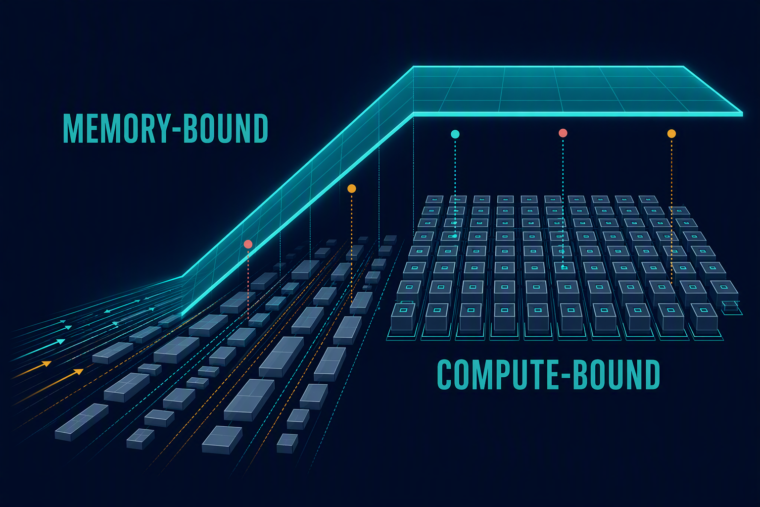
A sloped memory ceiling rising to meet a flat compute ceiling, with a marked corner between them.

Figure 1.2.1 — Throughput rises with reuse until it hits the arithmetic ceiling; everything left of the corner is a bandwidth problem wearing a compute problem's clothes.

Every kernel is a point under that roof. Its horizontal position comes from arithmetic — computable with no hardware present. Its vertical position comes from measurement. Confusing the two is how this model gets misused, because it gives you exactly two moves. Up: same algorithm, better execution — fix coalescing, pick a tensor-core kernel, stop launching tiny kernels. Right: same hardware, different algorithm — batch more rows through one weight read, fuse, shrink the elements. A point at intensity 1 cannot be rescued by a better kernel.

The mechanism¶

Count two things, and name the boundary¶

\[ I = \frac{\text{useful floating-point operations}}{\text{bytes crossing a named boundary}} \tag{1.2.1} \]

A FLOP is one operation under a stated convention: a multiply is one, an add is one, so a fused multiply-add is two — what every datasheet and scaling paper means, and the convention in NOTATION.md. A $(m \times k)$ by $(k \times n)$ multiply costs $2mkn$.

Bytes moved is traffic across a boundary you named out loud, not bytes your program allocated. The same function has low intensity against registers and high intensity against HBM, because a good kernel loads a tile once and hammers it on-chip — intensity is a property of a kernel at a boundary, never of a function. Traffic includes outputs: a kernel reading two 400-byte inputs, writing one 400-byte output, doing 2,400 FLOPs moves 1,200 bytes, so $I = 2$. Omit the write, report 3, and you have shifted the point 50% right into a different diagnosis.

The bound is one line, and the ceilings cross at the ridge:

\[ P(I) \;\le\; \min\!\left(P_{peak},\; B_{mem} \cdot I\right) \tag{1.2.2} \]

\[ I_{ridge} = \frac{P_{peak}}{B_{mem}} \tag{1.2.3} \]

Worked example — the ridge point, with the units done out loud

The A100 80 GB SXM delivers $P_{peak} = 312$ TFLOP/s of dense bf16 tensor-core throughput against $B_{mem} = 2.039$ TB/s. Both prefixes are $10^{12}$, so they cancel, and the seconds cancel:

\[ I_{ridge} = \frac{312 \times 10^{12}\ \text{FLOP/s}}{2.039 \times 10^{12}\ \text{byte/s}} = \frac{312}{2.039}\ \frac{\text{FLOP}}{\text{byte}} \approx \mathbf{153\ FLOP/byte} \]

For every byte the A100 fetches from HBM you must find 153 operations to perform on it, or the card cannot reach its advertised speed even in principle. 153 is the exchange rate between the two resources you rent, not a target. A kernel at $I = 10$ is capped at 20.4 TFLOP/s against an advertised 312 — 6.5%, and that is arithmetic, not engineering.

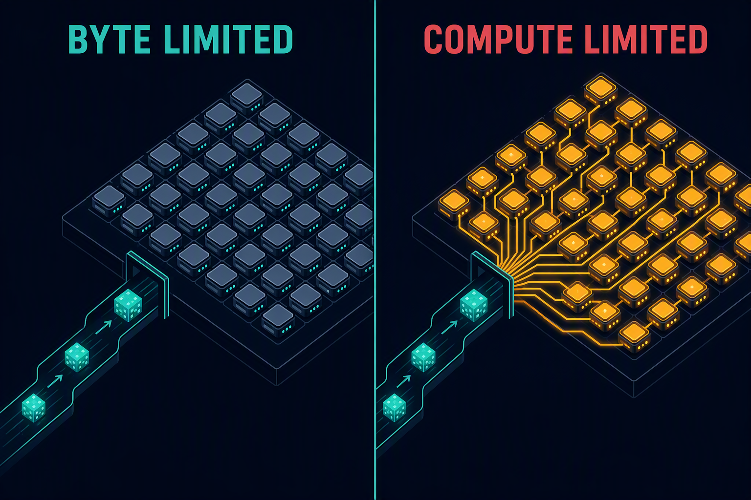
A starved arithmetic array waiting on a thin byte stream beside a saturated array fed by heavily reused blocks.

Figure 1.2.2 — Two ceilings, two failure modes: left, the units idle between deliveries; right, the deliveries are amortised and the units are the constraint.

One formula generates every case in this book¶

Nearly every heavy transformer operation is a weight matrix meeting some number of token rows. Take a $d \times d$ weight at $s$ bytes per element with $T$ rows in and out. Work is $2Td^2$; optimistic HBM traffic is the weight once plus input and output, $s(d^2 + 2Td)$: $$ I_{proj} = \frac{2Td^2}{s\,(d^2 + 2Td)} = \frac{2Td}{s\,(d + 2T)} \tag{1.2.4} $$

This is worth more than the graph. Its two limits, at $s = 2$:

$T \ll d$ (decode): the $d$ dominates and $I \to 2T/s = T$. Intensity is just the number of rows you batched.
$T \gg d$ (long prefill): the $2T$ dominates and $I \to d/s = 2048$. Projections have a compute-density ceiling set by model width and element size.

Worked example — how many rows does it take to reach the ridge?

Set $I_{proj} = 153$ with $d = 4096$, $s = 2$: $3790\,T = 626{,}688$, so $T \approx \mathbf{165}$.

You need roughly 165 token-rows sharing a single weight read before a Llama-3.1-8B projection is even theoretically capable of saturating an A100's tensor cores. That is why engines default --max-num-batched-tokens to 2,048 or 8,192 rather than 32, and why a decode-only batch — capped at a few dozen sequences before KV cache runs out — structurally cannot get there. Not a tuning parameter: model width divided by the card's exchange rate.

Where Llama-3.1-8B actually sits¶

Llama-3.1-8B has $N = 8.03$ B parameters, 14.96 GiB in bf16, and one token's forward pass costs approximately $2N$ FLOPs.

Worked example — decode at batch 1, the number that runs the industry

One decode step, one sequence, short context so KV traffic is negligible. Work: $2N = 1.61 \times 10^{10}$ FLOPs. Traffic: every weight, exactly once, $N \cdot s = 1.61 \times 10^{10}$ bytes.

\[ I_{decode} = \frac{1.61 \times 10^{10}\ \text{FLOP}}{1.61 \times 10^{10}\ \text{byte}} \approx \mathbf{1\ FLOP/byte} \]

Not approximately one — one, because bf16 spends two bytes to buy two FLOPs and every weight is used exactly once. The ridge is 153, so you are 153× to the left of it, and Equation 1.2.2 caps you at 2.04 TFLOP/s: 0.65% of the card's 312. A flawless decode kernel at batch 1 leaves 99.35% of the A100's arithmetic idle, and the step still takes at least 7.9 ms, because that is how long reading 14.96 GiB of weights takes.

Single-stream decode is not a compute workload that happens to be slow. It is a memory copy with a rounding error of arithmetic attached.

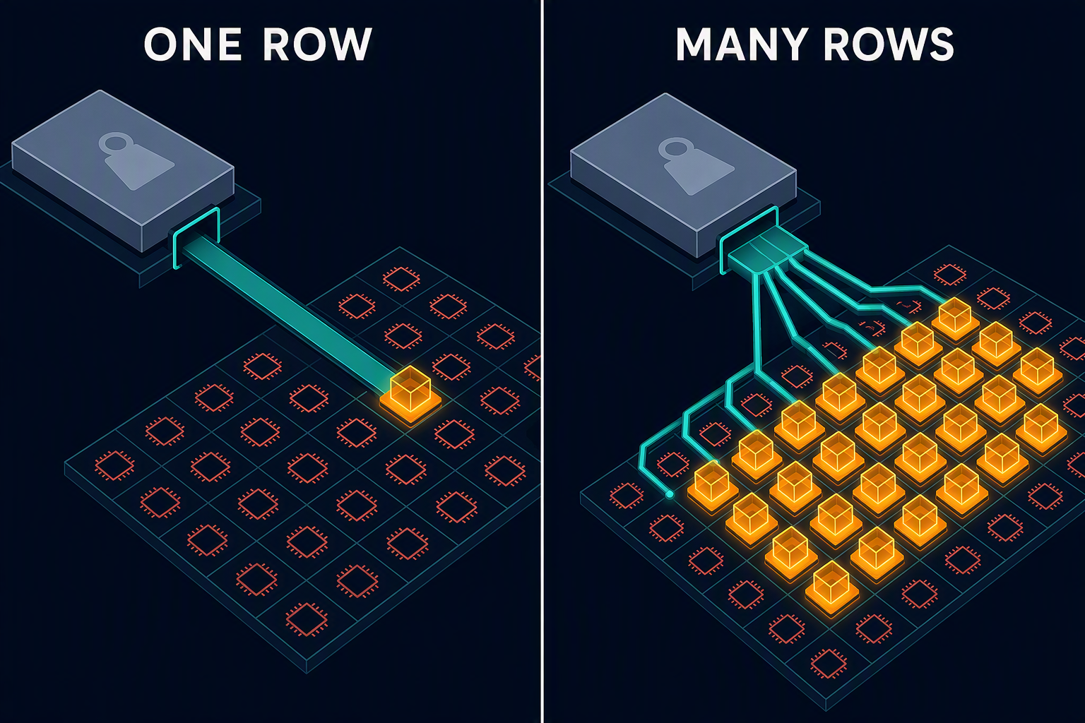
One weight slab feeding a single work item, beside the same slab feeding a dense stack of items.

Figure 1.2.3 — Batching does not make the weight read cheaper; it makes it serve more customers.

Worked example — batch 32, and the disappointment that follows

Thirty-two sequences, 2,048 tokens of context each. Work: $32 \times 2N = 5.14 \times 10^{11}$ FLOPs. Weights: still $1.61 \times 10^{10}$ bytes, read once and shared. KV: at 128 KiB per cached token (Chapter 2.2), $32 \times 2048 \times 131{,}072 = 8.59 \times 10^{9}$ bytes — not shared.

\[ I = \frac{5.14 \times 10^{11}}{1.61\times10^{10} + 8.59\times10^{9}} \approx \mathbf{21\ FLOP/byte} \]

Weights alone would give $I = 32$, exactly as Equation 1.2.4 predicts. A 21× efficiency gain for zero extra hardware is why continuous batching is the highest-leverage feature in any serving engine — and it is still 7× short of the ridge, capped at 14% of the card. KV traffic scales with the batch while weight traffic does not, so decode converges not on the ridge but on the cache's own ~1 FLOP/byte. Batching buys a lot and then stops buying.

Worked example — the same weights during a 4,096-token prefill

Change nothing but the row count. A 4,096-token prompt in one pass makes every projection a real GEMM. Equation 1.2.4 with $T = d = 4096$, $s = 2$:

\[ I_{prefill} = \frac{2 \times 4096 \times 4096}{2\,(4096 + 8192)} \approx \mathbf{1{,}365\ FLOP/byte} \]

Nine times to the right of the ridge. Same GPU, same weights, same process — now the memory system is comfortably ahead of the arithmetic units and 312 TFLOP/s is genuinely reachable. Chunk that prefill to 512 tokens and intensity falls to ≈ 410 FLOP/byte, still 2.7× right of the ridge, which is why chunked prefill caps TTFT spikes without surrendering compute efficiency.

Two phases, one model, opposite sides of the ridge, three orders of magnitude apart — the subject of Chapter 2.4, and the reason serious deployments run prefill and decode on separate pools: you are operating two machines that share a checkpoint.

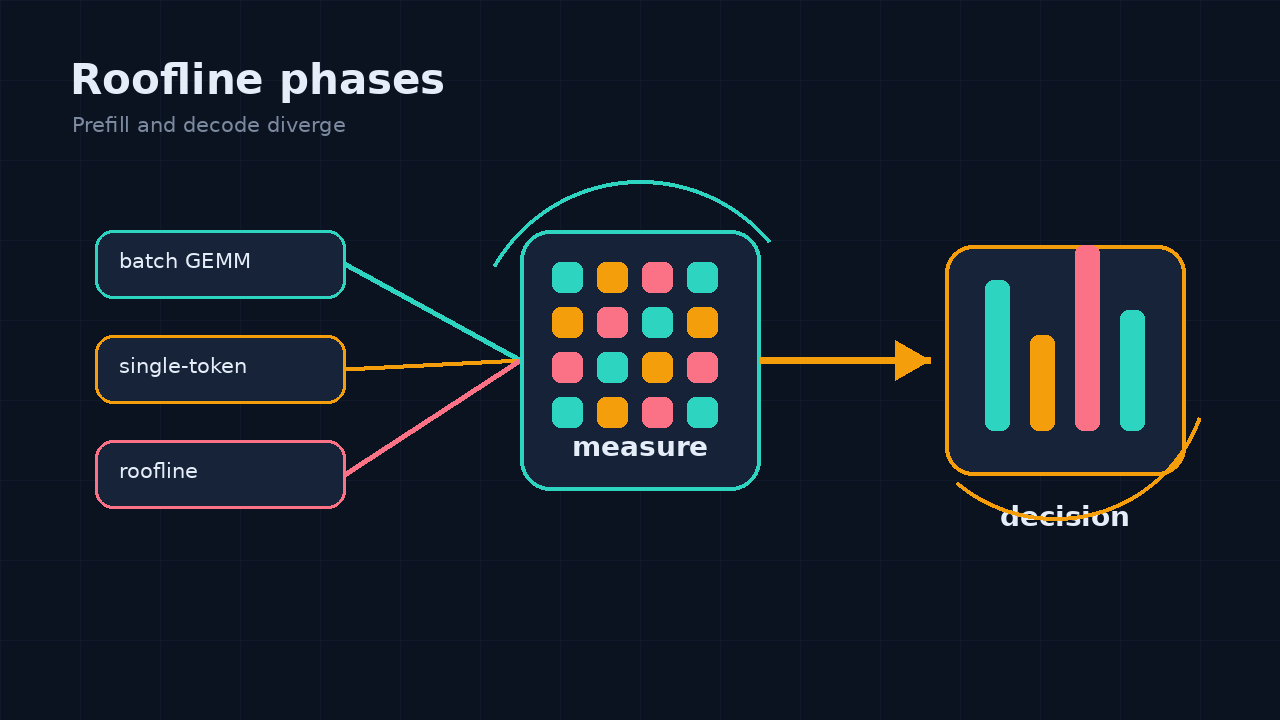
Two workloads placed on the same horizontal axis, one crowded far to the left of a marked corner and one far to the right.

Figure 1.2.4 — The distance between decode and prefill on this axis exceeds the distance between GPU generations. Hardware will not close it; scheduling might.

flowchart LR
    subgraph LEFT["Left of ridge — bandwidth business"]
        direction TB
        A["Decode, batch 1<br/>I ~ 1"]
        B["Decode, batch 32<br/>I ~ 21"]
        C["Norms, sampling, elementwise<br/>I &lt; 1"]
    end
    RIDGE{{"Ridge<br/>153 FLOP/byte<br/>A100 bf16"}}
    subgraph RIGHT["Right of ridge — arithmetic business"]
        direction TB
        D["Chunked prefill, 512 tokens<br/>I ~ 410"]
        E["Full prefill, 4096 tokens<br/>I ~ 1365"]
        F["Square GEMM, n = 8192<br/>I ~ 2730"]
    end
    A --> RIDGE
    B --> RIDGE
    C --> RIDGE
    RIDGE --> D
    RIDGE --> E
    RIDGE --> F

Where the transformer's operations land. Only one of these groups can use the tensor cores you rent.

Why a GEMM escapes and a decode step cannot¶

For $C = AB$ with $A$ of $m \times k$, $B$ of $k \times n$, $C$ of $m \times n$:

\[ I_{GEMM} \approx \frac{2mkn}{s\,(mk + kn + mn)} \tag{1.2.5} \]

Set $m = k = n$, $s = 2$. Work is $2n^3$; traffic is three $n \times n$ bf16 tensors, $6n^2$ bytes. So $I_{GEMM} \approx 2n^3/6n^2 = n/3$.

Cubic work over quadratic data. That asymmetry is why GEMM is the compute-bound operation and almost nothing else is: 1,365 at $n = 4096$, 2,730 at $n = 8192$. Growing the problem makes it more compute-dense. Decode collapses one dimension to 1, so a matrix-vector product does $2d^2$ FLOPs against $2d^2$ weight bytes and lands at intensity 1 forever, however large $d$ grows. You cannot reuse a byte you only need once.

Four ways to fabricate a wrong roofline

Undercounting bytes. Forgetting output writes, re-reads of an L2-evicted tensor, conversion buffers, or the $\beta C$ read in C = alpha*A@B + beta*C. Every omitted byte pushes the point right, toward "compute-bound", and hands you the wrong diagnosis.

Using the wrong peak. The A100's 312 TFLOP/s is bf16/fp16 tensor core; TF32 dense is 156, non-tensor FP32 is 19.5. Divide bf16 work by the FP32 peak and MFU inflates 16×.

Using the sparse peak. NVIDIA quotes 624 TFLOP/s for A100 bf16 with 2:4 structured sparsity. Dense inference cannot use it, so comparing against 624 silently halves every number you publish — and the error looks plausible enough to survive review.

MFU above 100%. Always a bug: sparse peak for dense work, FMA counted as one, or unsynchronised timing.

MFU and HFU answer different questions¶

\[ \mathrm{MFU} = \frac{\text{model FLOPs required} \;/\; \text{elapsed seconds}}{P_{peak}} \tag{1.2.6} \]

The numerator is what the model's mathematics demands, not what the GPU executed. Hardware FLOPs utilisation counts everything executed, including recomputation: with activation checkpointing HFU rises while MFU does not. Inference has the same trap in speculative-decoding rejects, padded batches, and masked positions — real arithmetic producing no tokens.

Judge MFU against the operation's own roofline ceiling, never against 100%.

Decode at batch 1 is capped at 0.65%, so escalating "0.6% MFU" is illiterate — it is 92% of the achievable bound. Meanwhile 40% MFU is good end-to-end, because that average includes attention, normalisation, sampling, collectives, and scheduler gaps, most of which live far left of the ridge. The same 40% on one large aligned bf16 GEMM is a bug, because that operation's ceiling is the flat roof.

A roof is a bound, not a prediction¶

Two kernels can share $I = 500$ and reach 80% and 25% of the roof; the model has nothing to say about the difference. Small matrices sit far below both ceilings because launch overhead and insufficient parallelism dominate before either resource is stressed. Awkward dimensions — a 128,256-wide vocabulary head — miss tensor-core tile shapes at identical theoretical intensity. Sustained clocks under load are not boost clocks.

A point sitting well beneath a roof line with a vertical gap marked between them.

Figure 1.2.5 — The horizontal position is arithmetic and you can trust it. The vertical gap to the roof is a profiler's job, not a roofline's.

flowchart TD
    A["Count useful FLOPs<br/>(FMA = 2)"] --> I["I = FLOPs / bytes<br/>at a named boundary"]
    B["Name the boundary<br/>(HBM unless stated)"] --> I
    C["Measured sustained bandwidth"] --> R["Ridge = P_peak / B_mem"]
    D["Dtype-matched dense peak"] --> R
    I --> Q{{"I below ridge?"}}
    R --> Q
    Q -- yes --> M["Memory-side<br/>ceiling = B_mem x I"]
    Q -- no --> P["Compute-side<br/>ceiling = P_peak"]
    M --> M2{{"Achieved near<br/>that ceiling?"}}
    P --> P2{{"Achieved near<br/>that ceiling?"}}
    M2 -- yes --> MX["Roofline is finished.<br/>Change the algorithm:<br/>batch, fuse, quantise"]
    M2 -- no --> PROF["Profiler question:<br/>coalescing, occupancy,<br/>launch overhead"]
    P2 -- yes --> PX["At the roof.<br/>Only more silicon helps"]
    P2 -- no --> PROF2["Profiler question:<br/>tile shape, kernel choice,<br/>clocks"]

The model routes you to one of two teams. Reaching the ceiling means the roofline is finished with you.

In practice¶

Build two rooflines whenever a diagnosis must survive an argument. The hardware roofline uses the SKU's published dense, dtype-matched peak and the sustained bandwidth you measured in Chapter 1.1 — not the spec sheet's 2.039 TB/s, which no real access pattern achieves. The empirical roofline uses the best your stack has demonstrated. The gap between roofs is platform opportunity; the gap between your point and the lower roof is kernel opportunity.

The code artifact states its assumptions rather than hiding them:

# [1] GEMM does 2n^3 FLOPs and minimally moves three n^2 tensors.
flops, bytes_moved = 2 * n**3, 3 * n**2 * a.element_size()

# [2] Ridge point: compute ceiling divided by memory-bandwidth ceiling.
ridge = compute * 1e12 / (bandwidth * 1e9)

"Minimally" is load-bearing: accumulate-into-C, cache eviction, or a conversion buffer all raise real traffic above what line [1] claims. Sweep production shapes too — $4096 \times 14336$ MLP projections, a $4096 \times 128{,}256$ vocabulary head, a batch-token dimension that changes every scheduler step. A roofline built only from friendly squares is a cuBLAS demonstration.

On newer silicon

Newer hardware moves the ridge right, which is worse than it sounds. An H100 SXM offers roughly 989 TFLOP/s dense bf16 against 3.35 TB/s of HBM3, giving $I_{ridge} \approx 295$ — nearly double the A100's. FP8 roughly doubles peak again to ~1,979 TFLOP/s while bandwidth does not move, pushing the ridge to $\approx 590$ FLOP/byte. Blackwell's FP4 path pushes it further.

Compute has outgrown bandwidth for a decade, so each generation makes more of your workload memory-bound, not less. Decode at intensity 1 does not improve on an H100; it fails to use an even larger fraction of a more expensive card.

The A100 is SM 8.0 and has no FP8 or FP4 tensor-core instructions at all — silicon, not software. Everything here is validated at bf16 and INT8 on Ampere. Know the FP8 ridge arithmetic for design reviews; do not put it in a capacity plan for this hardware.

Failure modes¶

Symptom	Cause	Fix
Nearly every kernel classifies as compute-bound	Bytes undercounted — outputs, re-reads, conversion buffers, accumulate-in-place traffic	Name the boundary, then enumerate every tensor crossing it. If the point moved right, you deleted traffic that exists
MFU above 100%	Sparse peak for dense work, FMA counted as one, unsynchronised timing, or non-model work in the numerator	Match dtype and sparsity mode; count FMA as two; synchronise before stopping the clock
A low-intensity kernel sits far below the sloped roof	Uncoalesced access, tiny transfers, launch overhead, or too little parallelism to saturate memory	Compare achieved bandwidth to Chapter 1.1's sustained number; sweep size before touching the math
A high-intensity GEMM sits far below the flat roof	Shape misses tensor-core tiles, a non-tensor-core kernel dispatched, or clocks throttled	Check dimension alignment, confirm the selected kernel in the profiler, log sustained clocks under load
Batching stops helping around 32–64 sequences	KV traffic scales with batch while weight traffic does not, so intensity asymptotes near the cache's own ~1 FLOP/byte	Model KV bytes explicitly (Chapter 2.2). Remaining levers are $H_{kv}$, cache dtype, context length — not batch size
Decode "only" reaches 1% MFU and is escalated as a regression	MFU judged against 100% instead of the operation's ceiling	Compute $B_{mem} \times I$. At $I = 1$ that is 0.65% of peak; you are at the bound, and the fix is batching, not kernels
Roofline says memory-bound but weight quantisation barely helps	Something other than weights dominates traffic — KV cache, activations, or a collective on the critical path	Break traffic down by tensor class before choosing an optimisation

Do it¶

Run the roofline artifact on the same quiet GPU you used for Chapter 1.1, passing the sustained bandwidth you measured there and the exact dense, dtype-matched peak for the precision under test.

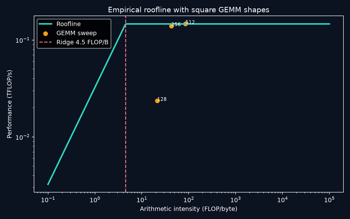
Measured GEMM points plotted beneath sloped and flat ceilings.

Figure 1.2.6 — The committed run here is labelled "device": "CPU diagnostic": 32.5 GB/s of bandwidth, 0.147 TFLOP/s of compute, a ridge of 4.5 FLOP/byte. It proves the plotting pipeline and the arithmetic, and it is not a GPU roofline. Replace it with your own CUDA run before citing it.

Success criterion. Three things, all objective:

Predict which side of the ridge each shape lands on before the sweep, and be right for every one.
Add three production shapes — the MLP projection, the vocabulary head, and one batch-token GEMM at your real max_num_batched_tokens — justifying each from Equation 1.2.4 or 1.2.5 before plotting.
For every point more than 30% below its ceiling, state a hypothesis and name the profiler counter that would confirm it.

Then compute your own deployment's decode intensity at its real batch size and the MFU ceiling that follows. If that ceiling is 14%, no kernel work will ever deliver the other 86%. LAB-M1 turns the clean sweep into a production-shaped test.

Summary¶

$I = \text{FLOPs} / \text{bytes across a named boundary}$. Without the boundary the number is meaningless.
$I_{ridge} = P_{peak}/B_{mem} \approx 153$ FLOP/byte on an A100: 153 operations per byte fetched, or the tensor cores cannot be saturated in principle.
A projection's intensity is $2Td/(s(d+2T))$, which is just $T$ when $T \ll d$. Llama-3.1-8B decode at batch 1 sits at $I \approx 1$ — 153× left of the ridge, capped at 0.65% of peak. Batch 32 reaches ~21 and is still 7× short. Roughly 165 rows per weight read are needed to touch the ridge.
The same weights during a 4,096-token prefill reach ~1,365 FLOP/byte. One model, two machines — which is why prefill and decode get scheduled separately.
The roofline is a bound, not a prediction. At the ceiling, change the algorithm; far below it, open a profiler. Judge MFU against the operation's own ceiling: 40% is excellent end-to-end, a bug for one GEMM.

Key terms¶

arithmetic intensity · ridge point · bandwidth-bound · compute-bound · MFU · HFU

Exercises¶

Recall

State the roofline bound and the ridge point in symbols, and say what "153 FLOP/byte" means physically.
Why is arithmetic intensity a property of a kernel at a boundary rather than of a function?

Derive

A GPU sustains 1.6 TB/s with a 240 TFLOP/s dense bf16 ceiling. Compute its ridge point. A kernel runs at $I = 12$: what is its maximum throughput, and what MFU is that?
Using Equation 1.2.4 with $d = 4096$, $s = 2$, compute intensity at $T = 8$, $T = 64$, $T = 512$. Which are within 3× of the A100 ridge?
Show that a square bf16 GEMM has $I \approx n/3$, then explain why decode can never reach that regime however wide the model becomes.

Design

You serve Llama-3.1-8B on one A100 80 GB. Decode runs at batch 24 with 4 K average context; the dashboard reads 6% MFU and an engineer proposes a two-week custom decode kernel. Compute the roofline ceiling, decide whether the project is justified, and rank three alternatives with their costs.

Worked solutions

**1.** $P(I) \le \min(P_{peak}, B_{mem} I)$ and $I_{ridge} = P_{peak}/B_{mem}$. Physically: every byte pulled from HBM must have 153 operations performed on it before the arithmetic units can run at their rated speed. Below that ratio the memory system sets the maximum. **2.** Numerator and denominator are counted in different places. FLOPs are fixed by the algorithm; bytes depend on the boundary. A tiled GEMM loads each HBM tile once and reuses it hundreds of times on-chip, so its HBM intensity is enormous while its register-level intensity is small. **3.** $I_{ridge} = 240/1.6 = \mathbf{150}$ FLOP/byte. At $I = 12$ the ceiling is 19.2 TFLOP/s, so $19.2/240 = \mathbf{8\%}$ MFU. A perfect implementation achieves 8%; anything near 8% is at the bound, and the only remaining move is to raise $I$. **4.** $I = 4096T/(4096 + 2T)$ gives $\mathbf{7.97}$, $\mathbf{62.1}$, and $\mathbf{409.6}$. The first two track the small-$T$ approximation $I \approx T$ to within 3%. Within 3× of the ridge means $I \ge 51$, so **$T = 64$ and $T = 512$ qualify**; $T = 512$ is past the ridge entirely. $T = 8$ is capped at 16 TFLOP/s. **5.** Work is $2n^3$; minimal traffic is three $n \times n$ bf16 tensors, $6n^2$ bytes, so $I = n/3$ — cubic work over quadratic data, so intensity grows without bound. Decode collapses one dimension to 1, making work $2d^2$ against $2d^2$ weight bytes, both quadratic, so the ratio is pinned at 1 for any $d$: each weight is needed once, and a byte used once cannot be reused. **6.** **Compute the ceiling before anyone writes code.** - Work: $24 \times 2N = 3.85 \times 10^{11}$ FLOPs per step - Weights: $1.61 \times 10^{10}$ bytes; KV: $24 \times 4096 \times 131{,}072 = 1.29 \times 10^{10}$ bytes - $I \approx \mathbf{13.3}$ FLOP/byte Ceiling $= 27.1$ TFLOP/s $= \mathbf{8.7\%}$ MFU at spec bandwidth, nearer **6.4%** at a realistic sustained 1.5 TB/s. The dashboard reads 6%. **The kernel project is not justified.** The workload is already at roughly 95% of its theoretical bound; a perfect kernel recovers a few percent of *its own ceiling*, not of the card. Ranked alternatives, all of which move the point *right*: 1. **Raise concurrency** — bigger batch, prefix caching, admission control. Free, but TPOT rises as KV traffic grows, and per the batch-32 example it saturates. 2. **Cut bytes with quantisation.** W8A8 or W4A16 roughly doubles intensity at the same batch; INT8 KV cache attacks the other term and buys concurrency. Cost: accuracy validation, and on Ampere INT8 is the ceiling since FP8 is unavailable. 3. **Enable chunked prefill** so decode steps ride along with a fat token budget, lifting the combined step past the ~165-row threshold. Cost: TTFT/TPOT tuning and scheduler complexity. When measured performance is close to the bound, change what the operation *is*, not how it is *implemented*.

Going deeper¶

Roofline: An Insightful Visual Performance Model for Multicore Architectures — the original; §3 on ceilings is still the clearest treatment
NVIDIA Nsight Compute — Roofline Charts — getting a hierarchical roofline out of a real kernel
PaLM: Scaling Language Modeling with Pathways — §5 defines MFU
Efficiently Scaling Transformer Inference — the decode intensity analysis these worked examples follow
NVIDIA A100 Tensor Core GPU Architecture — the dense and sparse peak tables you must not confuse

Next: Chapter 1.3 — Precision Formats, which attacks the same bound from the denominator: if you cannot find more FLOPs per byte, make each byte carry more of the model.